Entry
Reader's guide
Entries A-Z
Subject index
Taylor Series Linearization (TSL)
The Taylor series linearization (TSL) method is used with variance estimation for statistics that are vastly more complex than mere additions of sample values.
Two factors that complicate variance estimation are complex sample design features and the nonline-arity of many common statistical estimators from complex sample surveys. Complex design features include stratification, clustering, multi-stage sampling, unequal probability sampling, and without replacement sampling. Nonlinear statistical estimators for complex sample surveys include means, proportions, and regression coefficients. For example, consider the estimator of a subgroup total, 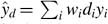 , where wi is the sampling weight, yi is the observed value, and di is a zero/one subgroup membership indicator for the ith sampling unit. This is a linear estimator because the estimate is a linear combination of the observed values yi and di. On the other hand, the domain mean,
 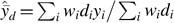 , is a nonlinear estimator as it is the ratio of two random variables and is not a linear combination of the observed data.
Unbiased variance estimation formulae for linear estimators are available for most complex sample designs. However, for nonlinear estimators, unbiased variance estimation formulae are often not available, and approximate methods must be used. The most common approximate methods are replication methods, such as the jackknife method or balanced repeated replication, and the TSL method.
The TSL method uses the linear terms of a Taylor series expansion to approximate the estimator by a linear function of the observed data. The variance estimation formulae for a linear estimator corresponding to the specifie sampling design can then be applied to the linear approximation. This generally leads to a statistical consistent estimator of the variance of a nonlinear estimator.
To illustrate the TSL method, let  be an estimate of the parameter θ where ŷ and ○ are two linear sample statistics. For example,
  . Also define μy and μx to be the expected values of ŷ and ○, respectively.
  can be expanded in a Taylor series expansion about μy and μx so that
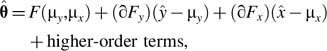
where ∂Fy and ∂FX are the first-order partial derivatives of F with respect to ŷ and ○ evaluated at their respective expectations, μy and μx. If the higher-order terms are negligible, then variance of can be approximated by
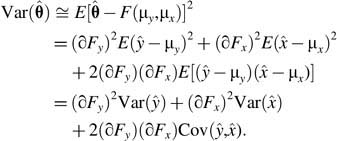
This approximation can easily be extended to functions of more than two linear sample statistics. An approximate estimate of the variance of is then obtained by substituting sample-based estimates of μy, μx, Var(ŷ) and Var(○) in the previous formula.
An equivalent computational procedure is formed by recognizing that the variable portion of the Taylor series approximation is 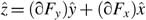 so that

Because ŷ and ○ are linear estimators, the Taylor series variance approximation can be computed using the linearized values 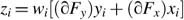 so that
  As before, substituting sample-based estimates of μy and μx, namely, ŷ and ○, in the formula for zi and then using the variance formula of a linear estimator for the sample design in question to estimate the variance of
  yields an approximate estimate of the variance of . This reduces the problem of estimating the variance of a nonlinear statistics to that of estimating the variance of the sum of the linearized values. As an example, the linearized values for the mean
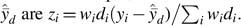
...
- Ethical Issues in Survey Research
- Anonymity
- Beneficence
- Cell Suppression
- Certificate of Confidentiality
- Common Rule
- Confidentiality
- Consent Form
- Debriefing
- Deception
- Disclosure
- Disclosure Limitation
- Ethical Principles
- Falsification
- Informed Consent
- Institutional Review Board (IRB)
- Minimal Risk
- Perturbation Methods
- Privacy
- Protection of Human Subjects
- Respondent Debriefing
- Survey Ethics
- Voluntary Participation
- Measurement - Interviewer
- Measurement - Mode
- Measurement - Questionnaire
- Aided Recall
- Aided Recognition
- Attitude Measurement
- Attitude Strength
- Attitudes
- Aural Communication
- Balanced Question
- Behavioral Question
- Bipolar Scale
- Bogus Question
- Bounding
- Branching
- Check All that Apply
- Closed-Ended Question
- Codebook
- Cognitive Interviewing
- Construct
- Construct Validity
- Context Effect
- Contingency Question
- Demographic Measure
- Dependent Variable
- Diary
- Don't Knows (DKs)
- Double Negative
- Double-Barreled Question
- Drop-down Menus
- Event History Calendar
- Exhaustive
- Factorial Survey Method (Rossi's Method)
- Feeling Thermometer
- Forced Choice
- Gestalt Psychology
- Graphical Language
- Guttman Scale
- HTML Boxes
- Item Order Randomization
- Item Response Theory
- Knowledge Question
- Language Translations
- Likert Scale
- List-Experiment Technique
- Mail Questionnaire
- Mutually Exclusive
- Open-Ended Question
- Paired Comparison Technique
- Precoded Question
- Priming
- Psychographic Measure
- Question Order Effects
- Question Stem
- Questionnaire
- Questionnaire Design
- Questionnaire Length
- Questionnaire-Related Error
- Radio Buttons
- Random Order
- Random Start
- Randomized Response
- Ranking
- Rating
- Reference Period
- Response Alternatives
- Response Order Effects
- Self-Administered Questionnaire
- Self-Reported Measure
- Semantic Differential Technique
- Sensitive Topics
- Show Card
- Step-Ladder Question
- True Value
- Unaided Recall
- Unbalanced Question
- Unfolding Question
- Vignette Question
- Visual Communication
- Measurement - Respondent
- Acquiescence Response Bias
- Behavior Coding
- Cognitive Aspects of Survey Methodology (CASM)
- Comprehension
- Encoding
- Extreme Response Style
- Key Informant
- Misreporting
- Nonattitude
- Nondifferentiation
- Overreporting
- Panel Conditioning
- Panel Fatigue
- Positivity Bias
- Primacy Effect
- Reactivity
- Recency Effect
- Record Check
- Respondent
- Respondent Burden
- Respondent Fatigue
- Respondent-Related Error
- Response
- Response Bias
- Response Latency
- Retrieval
- Reverse Record Check
- Satisficing
- Social Desirability
- Telescoping
- Underreporting
- Measurement - Miscellaneous
- Nonresponse - Item-Level
- Nonresponse - Outcome Codes and Rates
- Busies
- Completed Interview
- Completion Rate
- Contact Rate
- Contactability
- Contacts
- Cooperation Rate
- e
- Fast Busy
- Final Dispositions
- Hang-up during Introduction (HUDI)
- Household Refusal
- Ineligible
- Language Barrier
- Noncontact Rate
- Noncontacts
- Noncooperation Rate
- Nonresidential
- Nonresponse Rates
- Number Changed
- Out of Order
- Out of Sample
- Partial Completion
- Refusal
- Refusal Rate
- Respondent Refusal
- Response Rates
- Standard Definitions
- Temporary Dispositions
- Unable to Participate
- Unavailable Respondent
- Unknown Eligibility
- Unlisted Household
- Nonresponse - Unit-Level
- Advance Contact
- Attrition
- Contingent Incentives
- Controlled Access
- Cooperation
- Differential Attrition
- Differential Nonresponse
- Economic Exchange Theory
- Fallback Statements
- Gatekeeper
- Ignorable Nonresponse
- Incentives
- Introduction
- Leverage-Saliency Theory
- Noncontingent Incentives
- Nonignorable Nonresponse
- Nonresponse
- Nonresponse Bias
- Nonresponse Error
- Refusal Avoidance
- Refusal Avoidance Training (RAT)
- Refusal Conversion
- Refusal Report Form (RRF)
- Response Propensity
- Saliency
- Social Exchange Theory
- Social Isolation
- Tailoring
- Total Design Method (TDM)
- Unit Nonresponse
- Operations - General
- Advance Letter
- Bilingual Interviewing
- Case
- Data Management
- Dispositions
- Field Director
- Field Period
- Mode of Data Collection
- Multi-Level Integrated Database Approach (MIDA)
- Paper-and-Pencil Interviewing (PAPI)
- Paradata
- Quality Control
- Recontact
- Reinterview
- Research Management
- Sample Management
- Sample Replicates
- Supervisor
- Survey Costs
- Technology-Based Training
- Validation
- Verification
- Video Computer-Assisted Self-Interviewing (VCASI)
- Operations - In-Person Surveys
- Operations - Interviewer-Administered Surveys
- Operations - Mall Surveys
- Operations - Telephone Surveys
- Access Lines
- Answering Machine Messages
- Call Forwarding
- Call Screening
- Call Sheet
- Callbacks
- Caller ID
- Calling Rules
- Cold Call
- Computer-Assisted Telephone Interviewing (CATI)
- Do-Not-Call (DNC) Registries
- Federal Communications Commission (FCC) Regulations
- Federal Trade Commission (FTC) Regulations
- Hit Rate
- Inbound Calling
- Interactive Voice Response (IVR)
- Listed Number
- Matched Number
- Nontelephone Household
- Number Portability
- Number Verification
- Outbound Calling
- Predictive Dialing
- Prefix
- Privacy Manager
- Research Call Center
- Reverse Directory
- Suffix Banks
- Supervisor-to-interviewer Ratio
- Telephone Consumer Protection Act 1991
- Telephone Penetration
- Telephone Surveys
- Touchtone Data Entry
- Unmatched Number
- Unpublished Number
- Videophone Interviewing
- Voice over Internet Protocol (VoIP) and the Virtual Computer-Assisted Telephone Interview (CATI) Facility
- Political and Election Polling
- 800 Poll
- 900 Poll
- ABC News/Washington Post Poll
- Approval Ratings
- Bandwagon and Underdog Effects
- Call-in Polls
- Computerized-Response Audience Polling (CRAP)
- Convention Bounce
- Deliberative Poll
- Election Night Projections
- Election Polls
- Exit Polls
- Favorability Ratings
- FRUGing
- Horse Race Journalism
- Leaning Voters
- Likely Voter
- Media Polls
- Methods Box
- National Council on Public Polls (NCPP)
- National Election Pool (NEP)
- National Election Studies (NES)
- New York Times/CBS News Poll
- Poll
- Polling Review Board (PRB)
- Pollster
- Pre-Election Polls
- Pre-Primary Polls
- Precision Journalism
- Prior Restraint
- Probable Electorate
- Pseudo-Polls
- Push Polls
- Rolling Averages
- Sample Precinct
- Self-Selected Listener Opinion Poll (SLOP)
- Straw Polls
- Subgroup Analysis
- SUGing
- Tracking Polls
- Trend Analysis
- Trial Heat Question
- Undecided Voters
- Public Opinion
- Agenda Setting
- Consumer Sentiment Index
- Issue Definition (Framing)
- Knowledge Gap
- Mass Beliefs
- Opinion Norms
- Opinion Question
- Opinions
- Perception Question
- Political Knowledge
- Public Opinion
- Public Opinion Research
- Quality of Life Indicators
- Question Wording as Discourse Indicators
- Social Capital
- Spiral of Silence
- Third-Person Effect
- Topic Saliency
- Trust in Government
- Sampling, Coverage, and Weighting
- Adaptive Sampling
- Add-a-Digit Sampling
- Address-Based Sampling
- Area Frame
- Area Probability Sample
- Capture-Recapture Sampling
- Cell Phone Only Household
- Cell Phone Sampling
- Census
- Cluster Sample
- Clustering
- Complex Sample Surveys
- Convenience Sampling
- Coverage
- Coverage Error
- Cross-Sectional Survey Design
- Cutoff Sampling
- Designated Respondent
- Directory Sampling
- Disproportionate Allocation to Strata
- Dual-Frame Sampling
- Duplication
- Elements
- Eligibility
- Email Survey
- EPSEM Sample
- Equal Probability of Selection
- Error of Nonobservation
- Errors of Commission
- Errors of Omission
- Establishment Survey
- External Validity
- Field Survey
- Finite Population
- Frame
- Geographic Screening
- Hagan and Collier Selection Method
- Half-Open Interval
- Informant
- Internet Pop-up Polls
- Internet Surveys
- Interpenetrated Design
- Inverse Sampling
- Kish Selection Method
- Last-Birthday Selection
- List Sampling
- List-Assisted Sampling
- Log-in Polls
- Longitudinal Studies
- Mail Survey
- Mall Intercept Survey
- Mitofsky-Waksberg Sampling
- Mixed-Mode
- Multi-Mode Surveys
- Multi-Stage Sample
- Multiple-Frame Sampling
- Multiplicity Sampling
- n
- N
- Network Sampling
- Neyman Allocation
- Noncoverage
- Nonprobability Sampling
- Nonsampling Error
- Optimal Allocation
- Overcoverage
- Panel
- Panel Survey
- Population
- Population of Inference
- Population of Interest
- Post-Stratification
- Primary Sampling Unit (PSU)
- Probability of Selection
- Probability Proportional to Size (PPS) Sampling
- Probability Sample
- Propensity Scores
- Propensity-Weighted Web Survey
- Proportional Allocation to Strata
- Proxy Respondent
- Purposive Sample
- Quota Sampling
- Random
- Random Sampling
- Random-Digit Dialing (RDD)
- Ranked-Set Sampling (RSS)
- Rare Populations
- Registration-Based Sampling (RBS)
- Repeated Cross-Sectional Design
- Replacement
- Representative Sample
- Research Design
- Respondent-Driven Sampling (RDS)
- Reverse Directory Sampling
- Rotating Panel Design
- Sample
- Sample Design
- Sample Size
- Sampling
- Sampling Fraction
- Sampling Frame
- Sampling Interval
- Sampling Pool
- Sampling without Replacement
- Screening
- Segments
- Self-Selected Sample
- Self-Selection Bias
- Sequential Sampling
- Simple Random Sample
- Small Area Estimation
- Snowball Sampling
- Strata
- Stratified Sampling
- Superpopulation
- Survey
- Systematic Sampling
- Target Population
- Telephone Households
- Telephone Surveys
- Troldahl-Carter-Bryant Respondent Selection Method
- Undercoverage
- Unit
- Unit Coverage
- Unit of Observation
- Universe
- Wave
- Web Survey
- Weighting
- Within-Unit Coverage
- Within-Unit Coverage Error
- Within-Unit Selection
- Zero-Number Banks
- Survey Industry
- American Association for Public Opinion Research (AAPOR)
- American Community Survey (ACS)
- American Statistical Association Section on Survey Research Methods (ASA-SRMS)
- Behavioral Risk Factor Surveillance System (BRFSS)
- Bureau of Labor Statistics (BLS)
- Cochran, W. G.
- Council for Marketing and Opinion Research (CMOR)
- Council of American Survey Research Organizations (CASRO)
- Crossley, Archibald
- Current Population Survey (CPS)
- Gallup Poll
- Gallup, George
- General Social Survey (GSS)
- Hansen, Morris
- Institute for Social Research (ISR)
- International Field Directors and Technologies Conference (IFD&TC)
- International Journal of Public Opinion Research (IJPOR)
- International Social Survey Programme (ISSP)
- Joint Program in Survey Methodology (JPSM)
- Journal of Official Statistics (JOS)
- Kish, Leslie
- National Health and Nutrition Examination Survey (NHANES)
- National Health Interview Survey (NHIS)
- National Household Education Surveys (NHES) Program
- National Opinion Research Center (NORC)
- Pew Research Center
- Public Opinion Quarterly (POQ)
- Roper Center for Public Opinion Research
- Roper, Elmo
- Sheatsley, Paul
- Statistics Canada
- Survey Methodology
- Survey Sponsor
- Telemarketing
- U.S. Bureau of the Census
- World Association for Public Opinion Research (WAPOR)
- Survey Statistics
- Algorithm
- Alpha, Significance Level of Test
- Alternative Hypothesis
- Analysis of Variance (ANOVA)
- Attenuation
- Auxiliary Variable
- Balanced Repeated Replication (BRR)
- Bias
- Bootstrapping
- Chi-Square
- Composite Estimation
- Confidence Interval
- Confidence Level
- Constant
- Contingency Table
- Control Group
- Correlation
- Covariance
- Cronbach's Alpha
- Cross-Sectional Data
- Data Swapping
- Design Effects (deff)
- Design-Based Estimation
- Ecological Fallacy
- Effective Sample Size
- Experimental Design
- F-Test
- Factorial Design
- Finite Population Correction (fpc) Factor
- Frequency Distribution
- Hot-Deck Imputation
- Imputation
- Independent Variable
- Inference
- Interaction Effect
- Internal Validity
- Interval Estimate
- Intracluster Homogeneity
- Jackknife Variance Estimation
- Level of Analysis
- Main Effect
- Margin of Error (MOE)
- Marginals
- Mean
- Mean Square Error
- Median
- Metadata
- Mode
- Model-Based Estimation
- Multiple Imputation
- Noncausal Covariation
- Null Hypothesis
- Outliers
- p-Value
- Panel Data Analysis
- Parameter
- Percentage Frequency Distribution
- Percentile
- Point Estimate
- Population Parameter
- Post-Survey Adjustments
- Precision
- Probability
- Raking
- Random Assignment
- Random Error
- Raw Data
- Recoded Variable
- Regression Analysis
- Relative Frequency
- Replicate Methods for Variance Estimation
- Research Hypothesis
- Research Question
- Rho
- Sampling Bias
- Sampling Error
- Sampling Variance
- SAS
- Seam Effect
- Significance Level
- Solomon Four-Group Design
- Standard Error
- Standard Error of the Mean
- STATA
- Statistic
- Statistical Package for the Social Sciences (SPSS)
- Statistical Power
- SUDAAN
- Systematic Error
- t-Test
- Taylor Series Linearization
- Test-Retest Reliability
- Total Survey Error (TSE)
- Type I Error
- Type II Error
- Unbiased Statistic
- Validity
- Variable
- Variance
- Variance Estimation
- WesVar
- z-Score
- Loading...
Get a 30 day FREE TRIAL
-
 Watch videos from a variety of sources bringing classroom topics to life
 -
Read modern, diverse business cases
-
Explore hundreds of books and reference titles

Read next

More like this
Sage Recommends
We found other relevant content for you on other Sage platforms.
Have you created a personal profile? Login or create a profile so that you can save clips, playlists and searches