Statistical Power

The probability of correctly rejecting a null hypothesis that is false is called the statistical power (or simply, power) of the test. A related quantity is the Type II error rate (β) of the test, defined as the probability of not rejecting a false null hypothesis. Because power is based on the assumption that the null hypothesis is actually false, the computations of statistical power are conditional probabilities based on specific alternative values of the parameter(s) being tested. As a probability, power will range from 0 to 1 with larger values being more desirable; numerically, power is equal to 1 − β.

The statistical power is also related implicitly to the Type I error rate (∞), or significance level, of a hypothesis test. If ∞ is small, then it will be more difficult to reject the null hypotheses, implying that the power will also be low. Conversely, if ∞ is larger, then the null hypotheses will have a larger rejection region, and consequently the power will be larger. While power and Type I error rates do covary as these extremes suggest, the exact relationship between power and ∞ is more complex than might be ascertained by interpolating from these extreme cases.

Statistical power is usually computed during the design phase of a survey research study; typical values desired for such studies range from 0.70 to 0.90. Generally many survey items are to be compared across multiple strata or against some prior census value(s). For example, researchers may use data from the Current Population Survey to determine if the unemployment rate for California is lower than the national average. Power calculations can be computed for each questionnaire item, and the maximum sample size required to achieve a specified power level for any given question becomes the overall sample size. Generally, in practice, one or two key items of interest are identified for testing, or a statistical model relating several of the items as predictors and others as key independent variables is specified. Power calculations to determine the adequacy of target sample sizes are then derived for these specific questionnaire items or particular statistical tests of model parameters.

Consider a scenario involving a random-digit dialing sample of households selected to estimate the average food replacement costs after an extended power outage for the residents within a midwestern U.S. county. The average food loss cost per household based on data from previous storms was $500.00 (μ0). Because this particular storm was slightly more severe than a previous storm, officials believe that in actuality, the average food loss cost for households for the current storm is somewhere closer to $550.00 (μ1). The standard deviation of the distribution of food loss costs was assumed to be $100.00. The statistical power for the one-tailed hypothesis test based on a sample of 25 houses using a Type I error rate of 5% is to be computed. In this case, the particular effect size used in the computation of statistical power is Effect Size 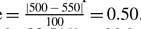. The statistical power for this test is 80.51%, which represents the [Page 845]probability of rejecting the null hypothesis of average food loss of $500.00 given that the actual average food loss costs is $550.00 using an estimated standard deviation of 100, a sample size of 25, and α = 0.05. Thus, there is roughly an 81% chance for detecting a positive difference in the average food loss costs of $50.00 using this hypothesis test. This power calculation is depicted graphically in Figure 1.

...