Standard Error of the Estimate

The standard error of the estimate (SEE) is, roughly speaking, the average “mistake” made in predicting values of the dependent variable (Y) from the estimated regression line. The SEE is assumed to be constant over all values of X. Thus, the average error in predicting Y when X = xi and X = xj, xi ≠ xj, will be the same. This is implied by the assumption of constant error variance [Var(ui|Xi) = σ2]in the classical linear regression model (CLRM).

There is an intuitive similarity between the SEE and the standard deviation of a random variable. The standard deviation of a random variable is nothing more than the square root of the average squared deviations from its mean. Similarly, the SEE is the square root of the average squared deviations from the regression line. Within a regression framework, these deviations are represented by the disturbance terms [Ûi = (yi − ŷi)]. Thus, the SEE can be understood as the standard deviation of the sampling distribution of disturbance terms, which, by assumption, is centered on zero. The SEE is also known as the root mean square error of the regression.

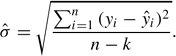
For a regression in which k parameters are estimated, where k is taken to be the number of independent variables in the regression model plus the constant, the SEE is given by the following:

[Page 1068]The SEE is a measure of the goodness of fit of the estimated regression line to the data. The smaller the SEE, the better the regression line fits the data. If the regression line fits the data perfectly, then each observation in the data set will fall exactly on the regression line and the SEE will be zero. Some researchers consider the SEE to be the preferred measure of fit of a regression model, and the statistic has many advantages. First, it is expressed in units of the dependent variable allowing for meaningful comparisons across regressions with the same dependent variable. Also, it is not dependent on the variance of the independent variables in the model as is another commonly used measure of fit, R2.

To see how the SEE is calculated, consider an example. An instructor is interested in predicting student performance in an introductory statistics class. The instructor believes that students' final exam grades are a linear additive function of the following independent variables: (a) GPA, (b) SAT, (c) Gender, and (d) Year in School. Using a random sample of 15 students, the instructor generates the following prediction equation:

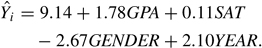
These estimates are then used to generate predicted values on Y for each of the students sampled (see Table 1).

How well does the estimated regression line fit the observed data? To answer this question, the instructor calculates the SEE. Using the data in Table 1 and the formula given above the SEE,

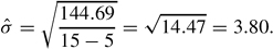
On average, the model will make a prediction error of 3.80 points. Recalling that a small standard error is associated with a better fit (and noting that the standard deviation of Y is 9.68), we would conclude that the estimated regression line fits the data in this example well.

...