ORDINARY LEAST SQUARES (OLS)

OLS Estimation

For example, consider the simple bivariate regression given by yi = β0 + β1xi + εi. The prediction equation is ŷi = β^0 + β^1xi. The residuals can be calculated as εi = yi − β^0 − β^1xi = yi − ŷi. Then the OLS estimator is defined by finding the minimum of the function S = ∑ni=1(yi − β^0 − β^1xi)2 with respect to the parameters β0 and β1. This is a concave quadratic function that always has a single minimum. This simple minimization problem can be solved analytically. The standard approach to minimizing such a function is to take first partial derivatives with respect to the two parameters β0 and β1, then solve the resulting set of two simultaneous equations in two unknowns. Performing these operations, we have the following:

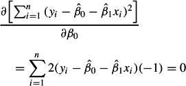
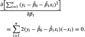
Simplifying this result and rearranging produces what are called the normal equations:

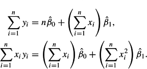
Because we can easily calculate the sums in the preceding equations, we have only to solve the resulting set of two simultaneous equations in two unknowns to have OLS estimates of the regression parameters. These analytical procedures are easily extended to the multivariate case, resulting in a set of normal equations specific to the dimension of the problem. For example, see Greene (2003, p. 21).

Classical Assumptions for OLS Estimation

The OLS estimator is incorporated into virtually every statistical software package and is extremely popular. The reason for this popularity is its ease of use and very convenient statistical properties. Recall that parameter estimation is concerned with finding the value of a population parameter from sample statistics. We can never know with certainty that a sample statistic is representative of a population parameter. However, using well-understood statistical theorems, we can know the properties of the estimators used to produce the sample statistics.

According to the Gauss-Markov theorem, an OLS regression estimator is a best linear unbiased estimator (BLUE) under the following assumptions.

• 1.
  The expected value of the population disturbances is zero (E[εi] = 0). This assumption implies that any variables omitted from the population regression function do not result in a systematic effect on the mean of the disturbances.
• 2.
  The expected value of the covariance between the population independent variables and disturbances is zero (E[Xi, εi] = 0). This assumption implies that the independent variables are nonstochastic, or, if they are stochastic, they do not covary systematically with the disturbances.
• 3.
  The expected value of the population correlation between disturbances is zero (E[εi, εj] = 0). This is the so-called nonautocorrelation assumption.
• 4.
  The expected value of the population variance of the disturbances is constant, (E[ε2i] = 0). This is the so-called non heteroskedasticity assumption.

These four assumptions about the population disturbances are commonly called the Gauss-Markov assumptions. Other conditions, however, are relevant to the statistical properties of OLS. If disturbances are normal, then the OLS estimator is the best unbiased estimator (BUE), but if disturbances are non-normal, then the OLS estimator is only the best linear unbiased estimator (BLUE). That is, another estimator that is either nonlinear or robust may be more efficient depending on the nature of the non-normality.

...