Nonparametric Random-Effects Model

Random-effects modeling is one of the several alternative approaches to deal with dependent observations such as those that occur in repeated measures or multilevel data structures. Nonparametric random effects models differ from standard (parametric) random effects models in that no assumptions are made about the distribution of the random effects. Actually, this is a form of LATENT CLASS ANALYSIS: The mixing distribution is modeled by means of a finite mixture structure. Early references to the nonparametric approach are Laird (1978) and Heckman and Singer (1982).

Let yij denote the response variable of interest, where the index j refers to a group and i to a replication within a group. Note that with repeated measures, groups and replications refer to individuals and time points. It is easiest to explain the random effects models within a GENERALIZED LINEAR MODELING framework; that is, to assume that the response variable comes from a distribution belonging to the exponential family and that the expectation of yij, E(yij), is modeled via a linear function after an appropriate transformation g[·].

A simple random intercept model without predictors has the following form:

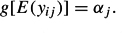
To utilize a parametric approach, a distributional form is specified for αj, typically normal: αj ∼ N(µ,τ 2). The unknown parameters to be estimated are the mean, µ, and the variance, τ 2. An equivalent parameterization is g[E(yij)] = µ+ τuj, with uj ∼ N(0, 1).

A nonparametric approach characterizes the distribution of αj by an unspecified discrete mixing distribution with C nodes (latent classes), where a particular latent class (LC) is enumerated by x,x = 1, 2, …,C. The intercept associated with class x is denoted by αx and the size of class x by P(x). The αx and P(x) are sometimes referred to as the location and weight of node x. The nonparametric model can be specified as follows:

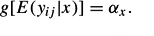
The nonparametric maximum likelihood estimator is obtained by increasing the number of latent classes until a saturation point is reached. In practice, however, researchers prefer solutions with less than the maximum number of classes.

The similarity between the parametric and nonparametric approaches becomes clear when one realizes that the αx and P(x) parameters can be used to compute the mean (µ) and the variance (τ 2) of the random effects, which are the unknown parameters in the parametric approach. Using elementary statistics, we get μ = ∑Cx = 1 αxP(x) and τ2 = ∑Cx = 1 (αx − μ)2P(x).

A more general model is obtained by including predictors zijk, yielding a two-level regression model with a random intercept:

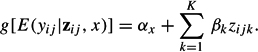
A special case is the (semiparametric) Rasch model, which is obtained by adding a dummy predictor for each replication i.

Also, the regression coefficient can be allowed to differ across latent classes, which is analogous to having random slopes in a MULTILEVEL ANALYSIS. This yields

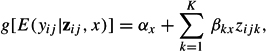
a model that is often referred to as a latent class (LC) or mixture regression model. In fact, this is one of the most important applications of latent class analysis: Unobserved subgroups are identified that differ with respect to the parameters of the regression model of interest.

...