Entry
Reader's guide
Entries A-Z
Subject index
Local Independence
Local independence is the basic assumption underlying LATENT VARIABLE models, such as FACTOR ANALYSIS, LATENT TRAIT ANALYSIS, LATENT CLASS ANALYSIS, and LATENT PROFILE ANALYSIS. The axiom of local independence states that the observed items are independent of each other, given an individual’s score on the latent variable(s). This definition is a mathematical way of stating that the latent variable explains why the observed items are related to one another.
We will explain the principle of local independence using an example taken from Lazarsfeld and Henry (1968). Suppose that a group of 1,000 persons are asked whether they have read the last issue of magazines A and B. Their responses are as follows:
| Table 1 | |||
|---|---|---|---|
| Read A | Did Not Read A | Total | |
| Read B | 260 | 240 | 500 |
| Did not read B | 140 | 360 | 500 |
| Total | 400 | 600 | 1,000 |
It can easily be verified that the two variables are quite strongly related to one another. Readers of A tend to read B more often (65%) than do nonreaders (40%). The value of phi coefficient, the product-moment correlation coefficient in a 2×2 table, equals 0.245.
Suppose that we have information on the respondents’ educational levels, dichotomized as high and low. When the 1,000 people are divided into these two groups, readership is observed in Table 2. Thus, in each of the 2 × 2 tables in which education is held constant, there is no association between the two magazines: the phi coefficient equals 0 in both tables. That is, reading A and B is independent within educational levels.
The reading behavior is, however, very different in the two subgroups: the high-education group has much higher probabilities of reading for both magazines (0.60 and 0.80) than the low-education group (0.20 and 0.20). The association between A and B can thus fully be explained from the dependence of A and B on the third factor, education. Note that the cell entries in the marginal AB table, N(AB), can be obtained by the following:
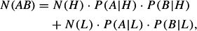
where H and L denotes high and low education, respectively.
In latent variable models, the observed variables are assumed to be locally independent given the latent variable(s). This means that the latent variables have the same role as education in the example. It should be noted that this assumption not only makes sense from a substantive point of view, but it is also necessary to identify the unobserved factors.
The fact that local independence implies that the latent variables should fully account for the associations between the observed items suggests a simple test of this assumption. The estimated two-way tables according to the model, computed as shown above for
| Table 2 | ||||||
|---|---|---|---|---|---|---|
| High Education | Low Education | |||||
| Read A | Did Not Read A | Total | Read A | Did Not Read A | Total | |
| Read B | 240 | 60 | 300 | 20 | 80 | 100 |
| Did not read B | 160 | 40 | 200 | 80 | 320 | 400 |
| Total | 400 | 100 | 500 | 100 | 400 | 500 |
N(AB), should be similar to the observed two-way tables. In the case of continuous indicators, we can compare estimated with observed correlations.
Variants of the various types of latent variable models have been developed that make it possible to relax the local independence assumption for certain pairs of variables. Depending on the scale type of the indicators, this is accomplished by inclusion of direct effects or correlated errors in the model.
- Analysis of Variance
- Association and Correlation
- Association
- Association Model
- Asymmetric Measures
- Biserial Correlation
- Canonical Correlation Analysis
- Correlation
- Correspondence Analysis
- Intraclass Correlation
- Multiple Correlation
- Part Correlation
- Partial Correlation
- Pearson's Correlation Coefficient
- Semipartial Correlation
- Simple Correlation (Regression)
- Spearman Correlation Coefficient
- Strength of Association
- Symmetric Measures
- Basic Qualitative Research
- Basic Statistics
- F Ratio
- N(n)
- t-Test
- X¯
- Y Variable
- z-Test
- Alternative Hypothesis
- Average
- Bar Graph
- Bell-Shaped Curve
- Bimodal
- Case
- Causal Modeling
- Cell
- Covariance
- Cumulative Frequency Polygon
- Data
- Dependent Variable
- Dispersion
- Exploratory Data Analysis
- Frequency Distribution
- Histogram
- Hypothesis
- Independent Variable
- Measures of Central Tendency
- Median
- Null Hypothesis
- Pie Chart
- Regression
- Standard Deviation
- Statistic
- Causal Modeling
- Discourse/Conversation Analysis
- Econometrics
- Epistemology
- Ethnography
- Evaluation
- Event History Analysis
- Experimental Design
- Factor Analysis and Related Techniques
- Feminist Methodology
- Generalized Linear Models
- Historical/Comparative
- Interviewing in Qualitative Research
- Latent Variable Model
- Life History/Biography
- Log-Linear Models (Categorical Dependent Variables)
- Longitudinal Analysis
- Mathematics and Formal Models
- Measurement Level
- Measurement Testing and Classification
- Multilevel Analysis
- Multiple Regression
- Qualitative Data Analysis
- Sampling in Qualitative Research
- Sampling in Surveys
- Scaling
- Significance Testing
- Simple Regression
- Survey Design
- Time Series
- ARIMA
- Box-Jenkins Modeling
- Cointegration
- Detrending
- Durbin-Watson Statistic
- Error Correction Models
- Forecasting
- Granger Causality
- Interrupted Time-Series Design
- Intervention Analysis
- Lag Structure
- Moving Average
- Periodicity
- Serial Correlation
- Spectral Analysis
- Time-Series Cross-Section (TSCS) Models
- Time-Series Data (Analysis/Design)
- Trend Analysis
- Loading...
Get a 30 day FREE TRIAL
-
 Watch videos from a variety of sources bringing classroom topics to life
 -
Read modern, diverse business cases
-
Explore hundreds of books and reference titles

Read next

More like this
Sage Recommends
We found other relevant content for you on other Sage platforms.
Have you created a personal profile? Login or create a profile so that you can save clips, playlists and searches