Least Squares

The least squares method—a very popular technique—is used to compute estimations of parameters and to fit data. It is one of the oldest techniques of modern statistics, being first published in 1805 by the French mathematician Legendre in a now-classic memoir. But this method is even older because it turned out that, after the publication of Legendre’s memoir, Gauss, the famous German mathematician, published another memoir (in 1809) in which he mentioned that he had previously discovered this method and used it as early as 1795. A somewhat bitter anteriority dispute followed (a bit reminiscent of the Leibniz-Newton controversy about the invention of calculus), which, however, did not diminish the popularity of this technique. Galton used it (in 1886) in his work on the heritability of size, which laid down the foundations of CORRELATION and (also gave the name) REGRESSION analysis. Both Pearson and Fisher, who did so much in the early development of statistics, used and developed it in different contexts (FACTOR ANALYSIS FOR PEARSON AND EXPERIMENTAL DESIGN for Fisher).

Nowadays, the least squares method is widely used to find or estimate the numerical values of the parameters to fit a function to a set of data and to characterize the statistical properties of estimates. It exists with several variations: Its simpler version is called ORDINARY LEAST SQUARES (OLS); a more sophisticated version is called WEIGHTED LEAST SQUARES (WLS), which often performs better than OLS because it can modulate the importance of each observation in the final solution. Recent variations of the least squares method are alternating least squares (ALS) and PARTIAL LEAST SQUARES (PLS).

Functional FIT Example: Regression

The oldest (and still most frequent) use of OLS was LINEAR REGRESSION, which corresponds to the problem [Page 560]of finding a line (or curve) that best fits a set of data. In the standard formulation, a set of N pairs of observations {Yi, Xi} is used to find a function giving the value of the dependent variable (Y) from the values of an independent variable (X). With one variable and a linear function, the prediction is given by the following equation:

This equation involves two free parameters that specify the intercept (a) and the slope (b) of the regression line. The least squares method defines the estimate of these parameters as the values that minimize the sum of the squares (hence the name least squares) between the measurements and the model (i.e., the predicted values). This amounts to minimizing the following expression:

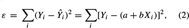
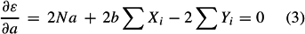
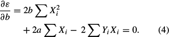
where ε stands for “error,” which is the quantity to be minimized. This is achieved using standard techniques from calculus—namely, the property that a quadratic (i.e., with a square) formula reaches its minimum value when its derivatives vanish. Taking the derivative of ε with respect to a and b and setting them to zero gives the following set of equations (called the normal equations):

and

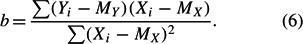
Solving these two equations gives the least squares estimates of a and b as

with MY and MX denoting the means of X and Y, and

OLS can be extended to more than one independent variable (using matrix algebra) and to nonlinear functions.

...