Latent Markov Model

The latent Markov model (LMM) can either be seen as an extension of the latent class model for the analysis of longitudinal data or as an extension of the discrete time Markov chain model for dealing with measurement error in the observed variable of interest. It was introduced in 1955 by Wiggins and also referred to as latent transition or the hidden Markov model. The LMM can be used to separate true systematic change from spurious change resulting from measurement error and other types of randomness in the behavior of individuals.

Suppose a single categorical variable of interest is measured at T occasions, and Yt denotes the response at occasion t,1 ≤ t ≤ T. This could, for example, be a respondent’s party preference measured at 6-month intervals. Let D denote the number of levels of each Yt, and let yt denote a particular level, 1 ≤ yt ≤ D. Let Xt denote an occasion-specific latent variable, C a number of categories of Xt, and xt a particular LC class at occasion t,1 ≤ xt ≤ C. The corresponding LMM has the form

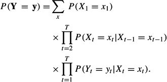
The two basic assumptions of this model are that the transition structure for the latent variables has the form of a first-order Markov chain and that each occasion-specific observed variable depends only on the corresponding latent variable. For identification and simplicity of the results, it is typically assumed that the error component is time homogeneous:

for 2 ≤ t ≤ T. If no further constraints are imposed, one needs at least three time points to identify the LMM. Typical constraints on the latent transition probabilities are time homogeneity and zero restrictions.

The enormous effect of measurement error in the study of change can be illustrated with a hypothetical example with T = 3 and C = D = 2. To illustrate this, suppose P(X1 = 1) = .80, P(Xt = 2|Xt−1 = 1) = P(Xt = 2|Xt−1 = 1) = .10, and P(Yt = 1|Xt = 1) = P(Yt = 2|Xt = 2) = .20. If we estimate a stationary manifest first-order Markov model for the hypothetical table, we find .68 in the first state at the first time point and transition probabilities of .29 and .48 out of the two states. These are typical biases encountered when not taking measurement error into account: The size of the smaller group is overestimated, the amount of change is overestimated, and there seems to be more change in the small than in the large group.

It is straight forward to extend the above single indicator LMM to multiple indicators. Another natural extension is the introduction of covariates or grouping variables explaining individual differences in the initial state and the transition probabilities. The independent classification error (ICE) assumption can be relaxed by including direct effects between indicators at different occasions. Furthermore, mixed variants of the LMM have been proposed, such as models with MOVER-STAYER structures. In social sciences, the LMM is conceived as a tool for categorical data analysis. However, as in standard LATENT CLASS ANALYSIS, these models can be extended easily to other scale types.

...