Intraclass Correlation

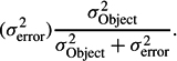
An intraclass correlation coefficient is a measure of association based on a variance ratio. Formally, it is the ratio of the variance for an object of measurement (σ2Object) to the object variance plus error variance:

It differs from an analog measure of association known as OMEGA SQUARED (ω2) only in the statistical model used to develop the sample estimate of σ2Object. Intraclass correlation estimates are made using the random effects model (i.e., the objects in any one sample are randomly sampled from a population of potential objects) and ω2 estimates are made using the FIXED EFFECTS MODEL (i.e., the objects in the sample are the only ones of interest and could not be replaced without altering the question being addressed in the research).

Intraclass correlation is best introduced using one of the problems it was developed to solve—what the correlation of siblings is on a biometric trait. If the sample used to obtain the correlation estimate consisted just of sibling pairs (in which sibships are the object of measurement), a Pearson product-moment, interclass correlation could be used, but this procedure would not lead to a unique estimate. The reason is seen with an example. For three sibling pairs {1, 2}, {3, 4}, and {5, 6}, the Pearson r for pairs when listed in this original order {1, 2}{3, 4}{5, 6} is different from the Pearson r for the same pairs if listed as {2, 1}{3, 4}{6, 5}, even though the sibling data are exactly the same. The Pearson procedure requires the totally arbitrary assignment of pair members to a set [Page 525]X and a set Y when, in fact, the only assignment is to sibship. How, then, is one to obtain a measure of correlation within sibship classes without affecting the estimate through arbitrary assignments? An early answer was to double-list each pair and then compute a Pearson r. For the example above, this meant computing the Pearson r for the twice-listed pairs {1, 2}{2, 1}{3, 4}{4, 3}{5, 6}{6, 5}.

Double-listing the data for each sibship leads to a convenient solution in the case of sibling pairs, but the method becomes increasingly laborious as sibships are expanded to include 3, 4, or k siblings. A computational advance was introduced by J. A. Harris (1913), and then R. A. Fisher (1925) applied his analysis of variance to the problem. This latter approach revealed that a sibling correlation is an application of the one-way random effects variance model. Inthismodel, each sibling value is conceptualized as the sum of three independent components: a population mean (μ) for the biometric trait in question; an effect for the sibship (α), which is a deviation of the sibship mean from the population mean; and a deviation of the individual sibling from the sibship mean (ε). In its conventional form, the model is written Yij = μ + αi + εij. The sibling correlation is then the variance of the alpha effects over the variance of the alpha effects plus epsilon (error) effects:

In other words, it is the proportion of total variance in the trait that is due to differences between sibships. For traits that run in families, the correlation would be high; for those that don't, the correlation would be low.

...