Heteroskedasticity

An assumption necessary to prove that the ORDINARY LEAST SQUARES (OLS) estimator is the BEST LINEAR UNBIASED ESTIMATOR (BLUE) is that the variance of the error is constant for all observations, or HOMOSKEDASTIC. Heteroskedasticity arises when this assumption is violated because the error variance is nonconstant. When this occurs, OLS parameter estimates will be unbiased, but the variances of the estimated parameters will not be efficient. A classic example is the regression of income on savings (Figure 1 provides a hypothetical visual example). We expect [Page 459]savings to increase as the level of income rises. This regression is heteroskedastic because individuals with low incomes have little money to save, and thus all have a relatively small amount of savings and small errors (they are all located near the regression line). However, individuals with high incomes have more to save, but some choose to use their surplus income in other ways (for instance, on leisure), so their level of savings varies more and the errors are larger.

Figure 1 Heteroskedastic Regression

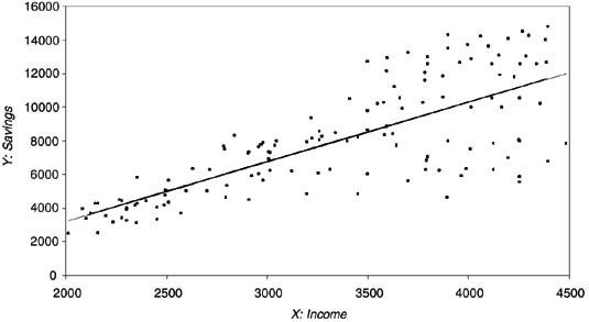
Figure 2 Visualizing Residuals

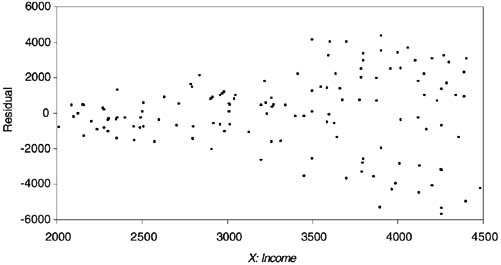
A number of methods to detect heteroskedasticity exist. The simplest is a visual inspection of the residuals Ûi = (yi −ŷi) plotted against each independent variable. If the absolute magnitudes of the residuals seem to be constant across values of all independent variables, heteroskedasticity is likely not a problem. If the dispersion of errors around the regression line changes across any independent variable (as Figure 2 shows it does in our hypothetical example), heteroskedasticity may be present. In any event, more formal tests for heteroskedasticity should be performed.

The Goldfeld-Quandt and Breusch-Pagan tests are among the options. In the former, the observations are ordered according to their magnitude on the offending variable, some central observations are omitted, and separate regressions are performed on the two remaining groups of observations. The ratio of their sum of squared residuals is then tested for heteroskedasticity. The latter test is more general, in that it does not require knowledge of the offending variable.

If the tests reveal the presence of heteroskedasticity, a useful first step is to again scrutinize the residuals to see if they suggest any omitted variables. It is possible that all over-predictions have a trait in common that could be controlled for in the model. In the example, a measure of the inherent value individuals place on saving money (or on leisure) could alleviate the problem. The high income-low savings individuals may value saving less (or leisure more) than the average individual. If no such change in model specification is apparent, it may be necessary to transform the variables and conduct a GENERALIZED LEAST SQUARES (GLS) estimation. The GLS procedure to correct for heteroskedasticity weights the observations on the offending independent variable by the inverse of their errors and is often referred to as WEIGHTED LEAST SQUARES (WLS). If the transformation is done, and no other regression assumptions are violated, transformed estimates are BLUE.