Bell-Shaped Curve

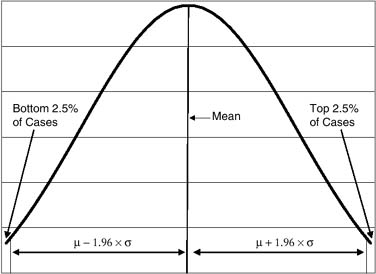
The bell-shaped curve is the term used to describe the shape of a normal distribution when it is plotted with the x-axis showing the different values in the distribution and the y-axis showing the frequency of their occurrence. The bell-shaped curve is a symmetric distribution such that the highest frequencies cluster around the midpoint of the distribution with a gradual tailing off toward 0 at an equal rate on either side in the frequency of values as they move away from the center of the distribution. In effect, it resembles a church bell, hence the name. Figure 1 illustrates such a bell-shaped curve. As can be seen from the symmetry and shape of the curve, all three MEASURES OF CENTRAL TENDENCY—the mean, the mode, and the median—coincide at the highest point of the curve.

The bell-shaped curve is described by its mean, μ, and its STANDARD DEVIATION, σ. Each bell-shaped curve with a particular μ and σ will represent a unique distribution. As the frequency of distributions is greater toward the middle of the curve and around the mean, the probability that any single observation from a bell-shaped distribution will fall near to the mean is much greater than that it will fall in one of the tails. As a result, we know, from normal probabilities, that in the bell-shaped curve, 68% of values will fall within 1 standard deviation of the mean, 95% will fall within roughly 2 standard deviations of [Page 61]the mean, and nearly all will fall within 3 standard deviations of the mean. The remaining observations will be shared between the two tails of the distribution. This is illustrated in Figure 1, where we can see that 2.5% of cases fall into the tails beyond the range represented by μ ± 1.96 × σ. This gives us the probability that in an approximately bell-shaped sampling distribution, any case will fall with 95% probability within this range, and thus, by statistical extrapolation, the population parameter can be predicted as falling within such a range with 95% confidence. (See also CENTRAL LIMIT THEOREM, NORMAL DISTRIBUTION.)

Figure 1 Example of a Bell-Shaped Curve

A particular form of the bell-shaped curve has its mean at 0 and a standard deviation of 1. This is known as the standard normal distribution, and for such a distribution the distribution probabilities represented by the equation μ ± z*σ simplify to the value of the multiple of σ (or Z-score) itself. Thus, for a standard normal distribution, the 95% probabilities lie within the range ±1.96.

Bell-shaped distributions, then, clearly have particular qualities deriving from their symmetry, such that it is possible to make statistical inferences for any distributions that approximate this shape. By extrapolation, they also form the basis of statistical inference even when distributions are not bell-shaped. In addition, distributions that are not bell-shaped can often be transformed to create an approximately bell-shaped curve. Thus, for example, income distributions, which show a skew to the right, can be transformed into an approximately symmetrical distribution by taking the log of the values. Conversely, distributions with a skew to the left, such as examination scores or life expectancy, can be transformed to approximate a bell shape by squaring or cubing the values.

...