Residual Plot

Concept

Defining a linear regression model as

the ith fitted value, the value lying on the hyper-plane, can be calculated as

where p refers to the number of explanatory variables and n the number of observations. For p = 1, the regression model represents a line; for p = 2, a plane; and for p = 3 or more, a hyper-plane. From here on, the term hyperplane is used, but the same concepts apply for a line, that is, for the simple regression model, or a plane.

The ith residual (ei), is then defined as

and it represents the vertical distance between the observed value (yi) and the corresponding fitted values (ŷi) for the ith observation. In this sense, the ith residual (ei) is an estimate for the unobservable error term (∊) and, thus, represents the part of the dependent variable (Y) that is not linearly related to the explanatory variables (X1, X2, …, Xp). One can also say that the ith residual (ei) is the part of Y that cannot be explained by the estimated regression model.

In regression analysis, the error terms incorporate a set of important and far-reaching assumptions. These are that the error terms are independently and identically distributed normal random variables, each with a mean of zero and [Page 1263]a common variance. This assumption can be expressed as

The residuals, however, do not necessarily exhibit these error term assumptions. By definition, for instance, the sum of all residuals must equal to zero, or

The direct implication from this residual property is that although the error terms are independent, the residuals are not. In addition, residuals resemble only estimates of the true and unobservable error terms and as such do not have the same variance σ2, as implied in Equation 4. The variance of the ith residual is defined as

where pii is the ith leverage value, that is, the ith diagonal element in the projection matrix, also known as the hat matrix. This unequal variance property can be coped with by means of standardization of the residuals.

Standardization of the residuals is achieved by dividing the ith residual by its standard deviation,

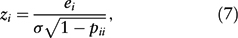
where zi denotes the ith standardized residual, which now by definition has a mean of zero and a standard deviation of one. For practical purposes, however, σ is not known and must therefore be replaced by the unbiased standard error of the estimate (

...