Poisson Distribution

Definition and Properties

The Poisson distribution is specified by a single parameter μ which determines the average number of occurrences of an event and takes any positive real number (i.e., μ > 0). When a random variable X, which can take all nonnegative integers (i.e., X = 0, 1, 2,…), follows the Poisson distribution with parameter μ, it is denoted by X ∼ Po(μ). The probability mass function of Po(μ) is given by

where e is the base of the natural logarithm (e = 2.71828…). The mean of X is μ, and the variance is also μ. The parameter μ is sometimes decomposed as μ = λt, where t is the length of a given time interval and λ denotes the “rate” of occurrences per unit time.

Figure 1 Probability Mass Functions of the Poisson Distributions With μ = 1, 5, and 10

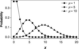
Figure 1 depicts the probability mass functions of the Poisson distributions with μ = 1, 5, and 10, respectively. The horizontal axis represents values of X, and the vertical axis represents the corresponding probabilities. When μ is small, the distribution is skewed to the right. As μ increases, however, the shape of distribution becomes more symmetric and its tails become wider.

The Poisson distribution arises as a result of the stochastic process called the Poisson process, which builds upon a set of postulates called the Poisson postulates. Roughly speaking, the Poisson postulates posit the following conditions on the probability of events occurring in given time intervals: (a) The numbers of events occurring in nonoverlapping time intervals are independent, (b) the probability of exactly one event in a very short (i.e., infinitesimally short) time interval is approximately proportional to the length of the interval, (c) the probability of more than one event in a very short interval is much smaller than the probability of exactly one event, and (d) the above probability structure is unchanged for any time interval. These postulates lead to a set of differential equations, and solving these equations for the probability of the number of events occurring in a given time interval produces the Poisson distribution.

The way by which the Poisson distribution is derived provides a basis for the distribution to be used for a model of rare events; the Poisson postulates state that the event occurs rarely within each small time interval but is given so many opportunities to occur. In this sense, the Poisson distribution is sometimes called the law of small numbers.

Relationship to Other Probability Distributions

The Poisson distribution is obtained as a limiting distribution of the binomial distribution with probability p and the number of trials n. Let μ = np, and increase n to infinity while μ is held constant (i.e., p approaches 0). The resulting distribution is Po(μ). This fact, in turn, implies that the Poisson distribution can be used to approximate the binomial distribution when n is large and p is small. This is of great use for calculating binomial probabilities when n is large, because the factorials involved in the binomial probability fomula become prohibitively large.

...