Factor Analysis: Exploratory

Introduction

Exploratory Factor Analysis (EFA) has long been a central technique in psychological research, as a powerful tool for reducing the complexity in a set of data. Its key idea is that the variability in a large sample of observed variables is dependent upon a restricted number of non-observable ‘latent’ constructs. This entry addresses key issues in EFA, such as: aims of EFA, basic equations, factor extraction and rotation, number of factors in a factor solution, factor measurement and replicability, assumptions, future perspectives.

Aims of Exploratory Factor Analysis

Exploratory Factor Analysis (EFA) has long been a central technique that has been widely used, since the beginning of the 20th century, in different fields of psychological research such as the study of mental abilities, of personality traits, of values and of beliefs, and the development of psychological tests (see Cattell, 1978; Comrey & Lee, 1992; Harman, 1976; McDonald, 1985). Its key idea is that the variability in a large sample of observed variables is dependent upon the action of a much-restricted number of non-observable ‘latent’ constructs. The aims of EFA are twofold: to reduce the dimensionality of the original set of variables, and to identify major latent dimensions (the factors) that explain the correlations among the observed variables. The starting point of an EFA is a matrix (R) of correlation coefficients (usually Pearson coefficients). The end is a matrix (A) that contains the correlations among the factors and the observed variables (called ‘factor loadings’): this is a rectangular matrix containing as many rows as the observed variables, and as many columns as the latent factors.

Basic Equations

The basic idea of EFA is that a standard score on a variable can be expressed as a weighted sum of the latent factors, so that the following specification equation holds:

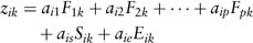
where zik is the standard score for a person k on the variable i; ai1 to aip, ais and aie are the loadings on, respectively, the common factors F, the specific factor S and the error factor E; F1k to Fpk, Sik and Eik are the standard scores of person k on, respectively, the common factors F, the specific factor S and the error factor E. While the common factors represent the variance that each variable shares with the other variables, the specific and error factors represent sources of variance that are unique for each variable.

The equation above is a basis for ‘decomposing’ the R matrix into the product of two other matrices, the matrix of factor loadings (A) and its transpose (A′), so that R = AA′ (this is called the fundamental equation of Factor Analysis). The key idea here is that the original correlation matrix can be ‘reproduced’ from the factor solution. From this decomposition it is possible to derive the following equation, which relates the variance of a standardized variable zi to the factor loadings:

In sum, the total variance of a standard variable can be divided into a part that each variable shares with the other variables and that is explained by the p common factors (this part is called communality, and is equal to the sum of squared loadings for the variable on the common [Page 404]factors, h2ii = a2i1 + a2i2 + … + a2ip) and a part that is explained by the specific and the error factors (the combination of these two components is called uniqueness, u2ii = a2is + a2ie).

...