Entry
Reader's guide
Entries A-Z
Subject index
Tuning Curves
The neurons within each sensory system must collectively encode the vast ranges of stimulus information that are environmentally relevant to the organism. A ubiquitous characteristic of neurons in all sensory systems, however, is their sensitivity to a wide range of stimulus parameters. That is, no single neuron is so selective that it is sensitive to just one single stimulus value. For example, in the auditory system, there will be no neuron that responds only to, say, middle C (∼262 hertz [Hz]) and no other sound frequencies. In order for each of the sensory systems to encode the ranges of possible stimulus parameters, the neurons comprising those systems divvy up the range such that each neuron exhibits differing selectivity, but over restricted ranges of those stimuli. For example, in the auditory system, the responses of neurons are often jointly sensitive to sound frequency and intensity, with different neurons encoding different ranges of frequency and intensity. The range of frequencies over which an auditory neuron is responsive is indicated by its tuning curve. In the visual system, peripheral neurons are differentially selective for the spatial location, luminance, and wavelength of the stimulus. This entry examines the concept of the tuning curve, which is an experimental measure of the selectivity of neurons in sensory systems to one or more stimulus parameters.
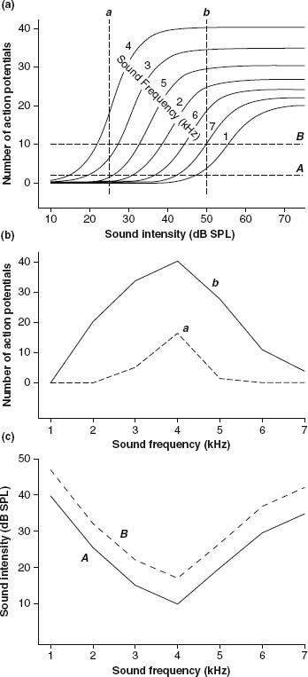
Figure 1 Example of a Tuning Curve
Measuring Tuning Curves
Figure 1 shows an example of how tuning curves are typically measured experimentally. Tuning curves can be measured as a function of one stimulus parameter or jointly as a function of two stimulus parameters. Here is a concrete example from the auditory system where tuning curves are often determined by measuring the number of action potentials a neuron fires (ordinate of Figure 1a) while varying the frequency (parameter of Figure 1a) and the intensity (abscissa of Figure 1a) of sounds presented to the ears. In many cases, the “responses” (action potentials in the current example) of the sensory systems being studied are related monotonically to monotonic increases in at least one stimulus parameter. This is particularly true for neurons or receptors at the most peripheral levels of a system.
It is important to keep in mind that quality and the quantity of the “response” being measured experimentally in the generation of a tuning curve can be of many different types. Most common of these is the number of action potentials a neuron under study fires in response to the presentation of a stimulus, such as in the example in Figure 1. The intracellular voltage (or current) potential of peripheral sensory receptors (e.g., hair cells, pho-toreceptors) and central neurons can also be used. These are just a few common types of responses that are measured in the generation of tuning curves.
...
- Action
- Action and Vision
- Corollary Discharge
- Echolocation
- Effort: Perception of
- Embodied Perception
- Event Perception
- Eye and Limb Tracking
- Eye Movements and Action in Everyday Life
- Eye Movements during Cognition and Conversation
- Eye Movements: Behavioral
- Eye Movements: Effects of Neurological and Mental Disorders On
- Feature Integration Theory
- Film (Cinema) Perception
- Guidance Systems for Blind People
- Haptics
- Human-Machine Interface
- Kinesthesia
- Mirror Neurons
- Motion Parallax and Structure from Motion
- Motion Perception
- Motion Perception: Social
- Multimodal Interactions: Visual-Haptic
- Navigation through Spatial Layout
- Perceptual Development: Imitation
- Perceptual Development: Touch and Pain
- Perceptual Development: Visually Guided Reaching
- Perceptual-Motor Integration
- Prism Adaptation
- Reaching and Grasping
- Response Time
- Self-Motion Perception
- Speech Production
- Tool Use
- Unconscious Processes
- Vestibular System
- Video Games
- Visual Search
- Visually Guided Actions
- Weight Perception
- Attention
- Attention and Consciousness
- Attention and Emotion
- Attention and Medical Diagnosis
- Attention and Memory
- Attention: Cognitive Influences
- Attention: Covert
- Attention: Cross-Modal
- Attention: Disorders
- Attention: Divided
- Attention: Effect of Breakdown
- Attention: Effect on Perception
- Attention: Object-Based
- Attention: Physiological
- Attention: Selective
- Attention: Spatial
- Attention: Theories of
- Bistable Perception
- Cell Phones and Driver Distraction
- Change Detection
- Consciousness
- Eye and Limb Tracking
- Eye Movements during Cognition and Conversation
- Film (Cinema) Perception
- Magic and Perception
- Perceptual Development: Attention
- Rapid Serial Visual Presentation
- Top-Down and Bottom-Up Processing
- Video Games
- Visual Search
- Audition
- Absolute Pitch
- Acoustics and Concert Halls
- Ageing and Hearing
- Agnosia: Auditory
- American Sign Language
- Animal Frequency and Pitch Perception
- Aphasias
- Audiology
- Audition
- Audition: Cognitive Influences
- Audition: Disorders
- Audition: Loudness
- Audition: Pitch Perception
- Audition: Temporal Factors
- Auditory Frequency Analysis, Neural
- Auditory Frequency Selectivity
- Auditory Illusions
- Auditory Imagery
- Auditory Localization: Physiology
- Auditory Localization: Psychophysics
- Auditory Masking
- Auditory Processing: Central
- Auditory Processing: Peripheral
- Auditory Receptors and Transduction
- Auditory Scene Analysis
- Auditory System: Damage Due to Overstimulation
- Auditory System: Evolution of
- Auditory System: Structure
- Auditory Thresholds
- Causality
- Cochlear Implants: Controversy
- Cochlear Implants: Technology
- Computer Speech Perception
- Computer-Generated Speech, Perception of
- Echolocation
- Evoked Potential: Audition
- Guidance Systems for Blind People
- Hearing Aids
- Language
- Lightning and Thunder
- Melody Perception
- Mirror Neurons
- Multimodal Interactions: Tactile-Auditory
- Multimodal Interactions: Visual-Auditory
- Music Cognition and Perception
- Music in Film
- Otoacoustic Emissions
- Perceptual Development: Hearing
- Perceptual Development: Infant Music Perception
- Perceptual Development: Intermodal Perception
- Perceptual Development: Speech Perception
- Sound Reproduction and Perception
- Sound Stimulus
- Speech Perception
- Speech Perception: Physiological
- Speech Production
- Speechreading
- Statistical Learning
- Synesthesia
- Timbre Perception
- Tinnitus
- Unconscious Processes
- Virtual Reality: Auditory
- Word Recognition
- Chemical Senses
- Ageing and Chemical Senses
- Air Quality
- Animal Chemical Sensitivity
- Aromatherapy
- Common Chemical Sense (Chemesthesis)
- Constancy
- Electronic Nose
- Flavor
- Fragrances and Perfume
- Multimodal Interactions: Color-Chemical
- Multimodal Interactions: Thermal-Chemical
- Olfaction
- Olfaction and Reproductive Behavior
- Olfaction: Evolution of
- Olfaction: Feature Detection and Integration
- Olfactometry
- Olfactory Adaptation
- Olfactory Bulb: Functional Architecture
- Olfactory Imagery
- Olfactory Localization
- Olfactory Quality
- Olfactory Receptors and Transduction
- Olfactory Stimulus
- Perceptual Development: Taste and Olfaction
- Pheromones
- Taste
- Taste Adaptation
- Taste and Food Preferences
- Taste Receptors and Transduction
- Taste Stimuli: Chemical and Food
- Taste System Structure
- Taste Thresholds and Intensity
- Taste: Disorders
- Taste: Genetics of
- Taste: Supertasters
- Visceral Perception
- Vomeronasal System
- Wine Tasting
- Cognition and Perception
- American Sign Language
- Attention and Medical Diagnosis
- Attention: Cognitive Influences
- Attention: Divided
- Attention: Selective
- Attention: Theories of
- Context Effects in Perception
- Cultural Effects on Visual Perception
- Decision Making, Perceptual
- Dyslexia
- Eye Movements during Cognition and Conversation
- Eyewitness Testimony
- Film (Cinema) Perception
- Language
- Magic and Perception
- Mind and Body
- Motion Perception: Social
- Music Cognition and Perception
- Music in Film
- Neural Prosthetic Systems
- Pain: Cognitive and Contextual Influences
- Recognition
- Sleep and Dreams
- Speech Perception
- Theory of Mind
- Time Perception
- Top-Down and Bottom-Up Processing
- Vision: Cognitive Influences
- Computers and Perception
- Consciousness
- Disorders of Perception
- Agnosia: Auditory
- Agnosia: Tactile
- Agnosia: Visual
- Amblyopia
- Aphasias
- Assistive Technologies for the Blind
- Attention: Disorders
- Auditory System: Damage Due to Overstimulation
- Body Perception: Disorders
- Cochlear Implants: Controversy
- Cochlear Implants: Technology
- Color Deficiency
- Consciousness: Disorders
- Cortical Reorganization following Damage
- Dyslexia
- Loss of a Sense: Effect on Others, Psychological
- Neural Prosthetic Systems
- Neuropsychology of Perception
- Olfaction: Disorders
- Pain: Treatments for Chronic
- Phantom Limb
- Prostheses: Visual
- Recovery of Vision following Blindness
- Sensory Rehabilitation
- Sensory Restoration and Substitution
- Speechreading
- Taste: Disorders
- Tinnitus
- Vision: Developmental Disorders
- Visual Disorders: Blindness
- Illusory Perceptions
- Individual Differences (Human) and Comparative (Across Species; Not Including Ageing, Disorders, and Perceptual Development)
- Absolute Pitch
- Animal Chemical Sensitivity
- Animal Color Vision
- Animal Depth Perception
- Animal Eye Movements
- Animal Eyes
- Animal Frequency and Pitch Perception
- Animal Motion Perception
- Cultural Effects on Visual Perception
- Echolocation
- Electroreception
- Emotional Influences on Perception
- Individual Differences in Perception
- Nature and Nurture in Perception
- Pain: Cognitive and Contextual Influences
- Perceptual Expertise
- Private Nature of Perceptual Experience
- Taste and Food Preferences
- Taste: Genetics of
- Taste: Supertasters
- Video Games
- Methods
- Brain Imaging
- Evoked Potential: Audition
- Evoked Potential: Vision
- Magnetoencephalography
- Microstimulation
- Neural Recording
- Neuropsychology of Perception
- Phenomenology (Philosophy)
- Physiological Approach
- Priming
- Psychophysical Approach
- Psychophysics: Detection
- Rapid Serial Visual Presentation
- Receptive Fields
- Recognition
- Response Time
- Reverse Correlation
- Scaling of Sensory Magnitude
- Selective Adaptation
- Signal Detection Theory and Procedures
- Transcranial Magnetic Stimulation
- Tuning Curves
- Visual Search
- Perceptual Development/Experience
- Ageing and Chemical Senses
- Ageing and Hearing
- Ageing and Touch
- Ageing and Vision
- Cultural Effects on Visual Perception
- Infant Perception
- Infant Perception: Methods of Testing
- Nature and Nurture in Perception
- Perceptual Development: Attention
- Perceptual Development: Color and Contrast
- Perceptual Development: Face Perception
- Perceptual Development: Hearing
- Perceptual Development: Imitation
- Perceptual Development: Intermodal Perception
- Perceptual Development: Object Perception
- Perceptual Development: Taste and Olfaction
- Perceptual Development: Touch and Pain
- Perceptual Development: Visual Acuity
- Perceptual Development: Visual Object Permanence and Identity
- Perceptual Development: Visually Guided Reaching
- Perceptual Expertise
- Perceptual Learning
- Prism Adaptation
- Statistical Learning
- Vision: Developmental Disorders
- Philosophical Approaches
- Causality
- Color: Philosophical Issues
- Computer Consciousness
- Consciousness
- Content of Perceptual Experience
- Indirect Nature of Perception
- Intentionality and Perception
- Inverted Spectrum
- Mary the Color Scientist
- Mind and Body
- Modality (Philosophy)
- Molyneux's Question
- Naïve Realism
- Perceptual Representation (Philosophy)
- Phenomenology (Philosophy)
- Philosophical Approaches
- Philosophy: Access and Report
- Philosophy: Attention and the Size of the Conscious Field
- Private Nature of Perceptual Experience
- Qualia
- Seeing As
- Visual Filling in and Completion
- Physiological Processes
- Aftereffects
- Binding Problem
- Contrast Enhancement at Borders
- Cortical Organization
- Cortical Reorganization following Damage
- Experience-Dependent Plasticity
- Feedback Pathways
- Lateral Inhibition
- Loss of a Sense: Effect on Others, Psychological
- Mirror Neurons
- Modularity
- Multimodal Interactions: Neural Basis
- Neural Prosthetic Systems
- Neural Recording
- Neural Representation/Coding
- Neuropsychology of Perception
- Oscillatory Synchrony
- Physiological Approach
- Receptive Fields
- Speed of Processing in Sensory Systems
- Tuning Curves
- Sense Interactions
- Action and Vision
- Attention: Cross-Modal
- Cortical Reorganization following Damage
- Cross-Modal Transfer
- Extrasensory Perception
- Flavor
- Loss of a Sense: Effect on Others, Psychological
- Molyneux's Question
- Motion Perception: Social
- Multimodal Interactions: Color-Chemical
- Multimodal Interactions: Neural Basis
- Multimodal Interactions: Pain-Touch
- Multimodal Interactions: Tactile-Auditory
- Multimodal Interactions: Thermal-Chemical
- Multimodal Interactions: Visual-Auditory
- Multimodal Interactions: Visual-Haptic
- Perceptual Development: Intermodal Perception
- Perceptual-Motor Integration
- Sensory Restoration and Substitution
- Synesthesia
- Taste and Food Preferences
- Skin and Body Senses
- Ageing and Touch
- Agnosia: Tactile
- Body Perception
- Body Perception: Disorders
- Braille
- Constancy
- Cutaneous Perception
- Cutaneous Perception: Physiology
- Electroreception
- Embodied Perception
- Haptics
- Itch, Tickle, and Tingle
- Kinesthesia
- Migraine
- Molyneux's Question
- Multimodal Interactions: Pain-Touch
- Multimodal Interactions: Tactile-Auditory
- Multimodal Interactions: Thermal-Chemical
- Multimodal Interactions: Visual-Haptic
- Out-of-Body Experience
- Pain: Assessment and Measurement
- Pain: Cognitive and Contextual Influences
- Pain: Neuromatrix Theory
- Pain: Physiological Mechanisms
- Pain: Placebo Effects
- Pain: Treatments for Chronic
- Perceptual Development: Touch and Pain
- Phantom Limb
- Proprioception
- Reaching and Grasping
- Surface and Material Properties Perception
- Tactile Acuity
- Tactile Map Reading
- Temperature Perception
- Texture Perception: Tactile
- Tool Use
- Vibratory Perception
- Virtual Reality: Touch/Haptics
- Visceral Perception
- Weight Perception
- Theoretical Approaches
- Bayesian Approach
- Computational Approaches
- Direct Perception
- Ecological Approach
- Embodied Perception
- Evolutionary Approach
- Evolutionary Approach: Perceptual Adaptations
- Gestalt Approach
- Indirect Nature of Perception
- Information Theory
- Physiological Approach
- Psychophysical Approach
- Theoretical Approaches
- Theory of Mind
- Visual Perception
- Action and Vision
- Aesthetic Appreciation of Pictures
- Aftereffects
- Afterimages
- Ageing and Vision
- Agnosia: Visual
- Amblyopia
- American Sign Language
- Ames Demonstrations in Perception
- Amodal Perception
- Animal Color Vision
- Animal Depth Perception
- Animal Eye Movements
- Animal Eyes
- Animal Motion Perception
- Assistive Technologies for the Blind
- Atmospheric Phenomena
- Attention and Consciousness
- Attention and Emotion
- Attention and Medical Diagnosis
- Attention: Cognitive Influences
- Attention: Covert
- Attention: Cross-Modal
- Attention: Disorders
- Attention: Divided
- Attention: Effect of Breakdown
- Attention: Effect on Perception
- Attention: Object-Based
- Attention: Physiological
- Attention: Selective
- Attention: Spatial
- Attention: Theories of
- Attractiveness
- Binding Problem
- Binocular Vision and Stereopsis
- Bistable Perception
- Camouflage
- Causality
- Change Detection
- Color Constancy
- Color Deficiency
- Color Mixing
- Color Naming
- Color Perception
- Color Perception: Physiological
- Color: Genetics of
- Color: Philosophical Issues
- Computer Graphics and Perception
- Computer Vision
- Constancy
- Context Effects in Perception
- Contrast Perception
- Corollary Discharge
- Depth Perception in Pictures/Film
- Digital Imaging
- Direct Perception
- Dyslexia
- Ecological Approach
- Embodied Perception
- Event Perception
- Evoked Potential: Vision
- Experience-Dependent Plasticity
- Eye and Limb Tracking
- Eye Movements and Reading
- Eye Movements during Fixation
- Eye Movements: Behavioral
- Eye Movements: Physiological
- Eye: Structure and Optics
- Eyes: Evolution of
- Eyewitness Testimony
- Face Perception
- Face Perception: Physiological
- Film (Cinema) Perception
- Gestalt Approach
- Impossible Figures
- Inverted Spectrum
- Lateral Inhibition
- Light Measurement
- Lightness Constancy
- Lightning and Thunder
- Linear and Nonlinear System Analysis
- Low Vision
- Magic and Perception
- Mary the Color Scientist
- McCollough Effect
- Mirages
- Mirror Neurons
- Molyneux's Question
- Motion Parallax and Structure from Motion
- Motion Perception
- Motion Perception: Physiological
- Motion Perception: Social
- Multimodal Interactions: Color-Chemical
- Multimodal Interactions: Visual-Auditory
- Multimodal Interactions: Visual-Haptic
- Navigation through Spatial Layout
- Neuropsychology of Perception
- Nonveridical Perception
- Object Perception
- Object Perception: Physiology
- Object Persistence
- Optic Ataxia
- Perception in Unusual Environments
- Perceptual Development: Face Perception
- Perceptual Development: Imitation
- Perceptual Development: Object Perception
- Perceptual Development: Visual Acuity
- Perceptual Development: Visual Object Permanence and Identity
- Perceptual Development: Visually Guided Reaching
- Perceptual Organization: Vision
- Perceptual Segregation
- Perceptual-Motor Integration
- Pictorial Depiction and Perception
- Prostheses: Visual
- Reaching and Grasping
- Reading Typography
- Recognition
- Recovery of Vision following Blindness
- Retinal Anatomy
- Sleep and Dreams
- Social Perception
- Spatial Layout Perception, Neural
- Spatial Layout Perception, Psychophysical
- Spatial Memory
- Speechreading
- Statistical Learning
- Surface and Material Properties Perception
- Texture Perception: Visual
- Unconscious Processes
- Video Games
- Virtual Reality: Vision
- Vision
- Vision: Cognitive Influences
- Vision: Developmental Disorders
- Vision: Temporal Factors
- Visual Acuity
- Visual Categorization: Physiological Mechanisms
- Visual Disorders: Blindness
- Visual Displays
- Visual Filling in and Completion
- Visual Illusions
- Visual Imagery
- Visual Light- and Dark-Adaptation
- Visual Masking
- Visual Memory
- Visual Processing: Extrastriate Cortex
- Visual Processing: Primary Visual Cortex
- Visual Processing: Retinal
- Visual Processing: Subcortical Mechanisms for Gaze Control
- Visual Receptors and Transduction
- Visual Scene Perception
- Visual Scene Statistics
- Visual Search
- Visual Spatial Frequency Analysis
- Visual Stimuli
- Visual System Structure
- Visual System: Evolution of
- Visually Guided Actions
- Word Recognition
- Loading...
Get a 30 day FREE TRIAL
-
 Watch videos from a variety of sources bringing classroom topics to life
 -
Read modern, diverse business cases
-
Explore hundreds of books and reference titles

Read next

More like this
Sage Recommends
We found other relevant content for you on other Sage platforms.
Have you created a personal profile? Login or create a profile so that you can save clips, playlists and searches