Structural Equation Modeling

Structural equation modeling (SEM) is a very general statistical approach for modeling and estimating data. It is seen as a combination of factor analysis and regression or path analysis. These procedures are regarded as special cases of SEM. It contains, in addition, classical multivariate [Page 2553]techniques such as analysis of variance, analysis of covariance, dummy regression, and canonical correlation as special cases. A structural equation model contains latent variables that should correspond to theoretical constructs from substantive theory and their reflective indicators or items that form the measurement model. The relationships between the latent variables (constructs and factors) and their indicators (observed variables) are quantified by the corresponding factor loadings. The regression coefficients between the latent variables (structural relations) take random and nonrandom measurement error into account and are, therefore, not biased. This part of the model is called “structural model” and represents the underlying theory. This entry presents some of the basic features of SEM using an example from the European Social Survey (ESS).

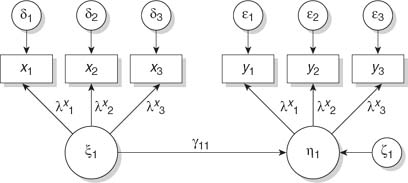
SEM models can be visualized by a graphical path diagram, which represents the relationships between the latent variables (structural model) and the relationships between latent and observed variables (measurement model). The latent variables are symbolized by circles, the observed variables by rectangles, and the postulated direction of influences by directed arrows (see Figure 1). The path diagram can be translated into a set of linear or matrix equations. Figure 1 displays a diagram that graphically represents a structural equation model with the measurement and the structural part. It contains one exogenous (independent) construct and one endogenous (dependent) construct. Each construct in Figure 1 is measured by three indicators to control for all forms of random and non-random measurement errors.

In Figure 1, ξ1 is an exogenous latent construct, measured by three indicators x1, x2, and x3. Their measurement errors are designated as δ1, δ2, and δ3. η1 is an endogenous latent construct, measured by three indicators y1, y2, and y3. Their measurement errors are designated as ε1, ε2, and ε3. λ is the symbol for the unstandardized factor loading. The residual of the latent endogenous variable is ζ1. It represents the unexplained variance of the latent endogenous variable. The regression coefficient between the exogenous and the endogenous latent variable is Γ11. The first subscript refers to the dependent variable, the second to the independent variable.

The corresponding equation system for the model in Figure 1 is as follows:

Structural model:

Measurement model:

The intercepts of the structural and the measurement model have been omitted.

Figure 1 The General Model for Two Latent Variables

The items are conceptualized as reflective indicators, as in confirmatory factor analysis, which means that the researcher postulates a direction of influence from the latent to the observed variable. Both the measurement model and the structural model can be generalized to take into account n indicators and m constructs. One can now differentiate between three types of parameters: (1) free parameters to be estimated from the data, such as in classical multivariate analysis; (2) fixed parameters that are set a priori to a certain value such as 0 or 1; and (3) constrained parameters that are set equal to another parameter. For estimating the coefficients, several estimation methods are available. The standard method is maximum likelihood estimation. By using this method, all the free parameters are estimated simultaneously taking into account both the fixed and the constrained parameters in the minimization of the fitting function. Other estimation methods take nonnormal distributions into account such as robustified maximum likelihood, asymptotic distribution free estimator (ADF), and weighted least squares (WLS). In addition, Bayesian estimation is possible, which allows the testing of a broader class of hypotheses and which may be more robust in smaller samples. The model testing is mostly done in at least two steps, because otherwise the necessary model modifications are too complex.

...