Statistical Inference, Classical and Bayesian

Statistical inference is a form of induction and can be broadly defined as “learning from data.” The two dominant forms of statistical inference are “classical” (or “frequentist”) inference and Bayesian inference.

Briefly, classical inference assesses the plausibility of a hypothesis by asking how frequently we would see results like the one actually obtained in repeated applications of the data generation mechanism, assuming the hypothesis to be true. If a statistic computed with the observed data is judged to be sufficiently unusual relative to its expected value under the hypothesis, then the hypothesis is considered falsified. The assumed hypothesis is often a “null” or “no effects” hypothesis; if this hypothesis is rejected (in the sense given above), then we usually say that we have a “statistically significant” finding. The assumptions here are that statistics vary randomly across repeated applications of the data generation mechanism (e.g., random sampling, say in the case of the analysis of survey data), while the objects of interest—population parameters θ—are constants. Repeated applications of the sampling process, if undertaken, would yield different y and different. The distribution of values of that would result from repeated applications of the sampling process is called the sampling distribution of; the standard deviation of this distribution is the standard error of. For many statistics, asymptotic theory gives the form of the statistic's large-sample sampling distribution (e.g., normal, χ2). The sampling variance of a statistic is often also easy to estimate; for instance, if is the maximum likelihood estimate, then V() is often estimated with the inverse of the information matrix (minus the second derivatives of the log of the likelihood function with respect to θ, usually evaluated either at or at a hypothesized value θ∗). This approach is by and far the most frequently taught and frequently deployed framework for statistical inference in the social sciences.

By contrast, Bayesian inference uses Bayes rule (we will drop the apostrophe in “Bayes' rule”) to compute the conditional probability of hypotheses given the data at hand, without any explicit reference to what might happen over repeated applications of the data generation mechanism. Bayes rule states that if A and B are events then

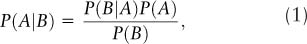
where P(A|B) is the conditional or posterior probability of A given that event B has occurred, P(A) is the prior probability of A, and P(B) is the marginal probability of B. This proposition—an uncontroversial result given the conventional definition of conditional probability—can be restated more provocatively as

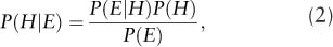
where P(H) is the prior probability of a hypothesis and P(E|H) is the likelihood of “evidence” (or data) E under hypothesis H. This form of Bayes rule underscores its relevance as a tool for statistical inference. In the case of a finite set of competing hypotheses H = {H1, …, Hj}, the law of total probability implies that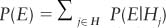P(Hj). Note that the resulting posterior probabilities constitute a proper probability mass function over the set H; that is, . For the case of a continuous parameter and data y ∼ p(y|θ), Bayes rule becomes

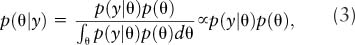
or (in words) the posterior density for θ is proportional to the prior density for θ, p(θ), times the likelihood for the data given 0, p(y| θ). The integral in the denominator in Equation 3 ensures that the posterior density integrates to one and thus is a proper probability density.

...