Monte Carlo Methods

Monte Carlo methods describe a set of computer simulation techniques that rely on random number generation to solve complex optimization and integration problems arising in statistics and its related fields. The term Monte Carlo is a reference to the probabilistic rules underlying casino games of chance, and though the theoretical underpinnings for their use emerged in the postwar period, it is the advent of inexpensive, modern computing that enabled their widespread adoption for practical problem solving.

Typically presented as an alternative to time-consuming analytical efforts, Monte Carlo methods allow researchers more freedom to posit models and make more subtle inferences from them—that is, they no longer need to rely on standard, but unrealistic, assumptions about complex (causal) processes that ensure a tractable solution exists. [Page 1627]This has proved particularly important in Bayesian analysis, where quantities of interest are available in principal by complex integration operations, yet can be (well) approximated via simulation. Precisely because such techniques have proved popular in political science, this integration aspect of Monte Carlo methods is the focus here. This entry begins with a discussion of the basic integration operation; then, it moves to the importance of random number generation and methods of sampling before considering Markov chain Monte Carlo methods. This latter set of techniques has proved extremely popular in political science over the past 10 years or so, especially for applying item–response models to obtain “ideal points” from roll call data. There are also large literatures dealing with optimization via Monte Carlo procedures and integration via (nonsimulation) deterministic numerical approaches; these are not discussed here.

Classical Monte Carlo Integration

To keep matters simple, consider the evaluation of the following integral:

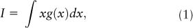
where g(x) is a probability density function. As presented, the integral will yield the expectation of the random variable X denoted E(X). But performing the operation may be difficult, perhaps because the integral has no closed form. A helpful alternative to this effort is to generate a sample of size m from the density g(x) and then to compute the empirical average,

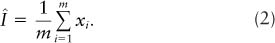
As m increases, by the strong law of large numbers, Î converges almost surely to the true value of I—and thus, the true value of E(X). Denoted the Monte Carlo method, the idea is more general. We can replace x in Equation 1 with some arbitrary function of x, denoted h(x). This might be the median or some other percentile. And we can assess definite integrals so long as we can produce a sample of x values between the specified bounds.

The variance of Î is decreasing in m. When var(m) is finite, the central limit theorem applies as the sample size increases, and we can place bounds on our estimates. Moreover, asymptotically, it is possible to obtain quantities that can be used to assess convergence directly.

This simulated integration takes on an important role in Bayesian statistics, since we often want to perform a variant on Equation 1. In particular, we are concerned with characteristics—such as the mean or median—of the posterior distribution π(θ|y), where θ is an unknown parameter and y the observations. In that case, we

...