Hypothesis Testing

The Current Paradigm: Null Hypothesis Significance Testing

The current approach to hypothesis testing in all of the social sciences is a synthesis of the Fisher test of significance and the Neyman-Pearson hypothesis test. In this 20th-century procedure, two hypotheses are set forth: a null or restricted hypothesis, H0, which is set against an alternative [Page 1117]or research hypothesis, H1. Thus, they are supposed to describe two complementary notions about some political science phenomenon of interest. The research hypothesis is the probability model that describes the author's belief about this phenomenon and is typically operationalized through statements about an unknown parameter θ ∊ Θ. In the most basic and common setup, the null hypothesis asserts that θ = 0, and the research hypothesis asserts that θ ≠ 0. Such a two-sided test is the overwhelming default in assessing the statistical reliability of individual regression parameters.

Once the hypotheses are established, a test statistic T, some function of θ and the data, is calculated and assessed with the distribution under the assumption that H0 is true. Commonly used test statistics are sample means, chi-square statistics from tabular analysis, χ2; and t statistics in linear and generalized linear models. Note that the sample space of the test statistic must correspond to the support of the specified null and alternative distributions. The key idea is that test statistics that appear to be “unusual” for the null distribution (e.g., those in the tails) cast doubt on the original assumption that this is the true distribution.

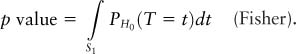
The test procedure ϕ assigns one of two decisions, D0 and D1, to all possible values in the sample space of the statistic T, corresponding to supporting either H0 or H1, respectively. The p value (also called the associated probability) is equal to the area in the tail (or tails) of the assumed distribution under H0, which starts at the point determined by T on the horizontal axis and continues to positive or negative infinity. If a predetermined significance level α has been specified, then H0 is rejected for p values less than α; otherwise, the p value itself is reported. More formally, the sample space of T is split into two complementary regions, S0 and S1, such that the probability that T falls in S1, causing decision D1, is either a predetermined null hypothesis cumulative distribution function (CDF) level (α = size of the test, Neyman-Pearson) or the CDF level corresponding to the value of the test statistic under H0 is reported as follows:

Thus, decision D1 is made if the test statistic is sufficiently atypical given the distribution under H0. This process is illustrated for a one-tailed test at α = .05 in Figure 1.

...