Entry
Reader's guide
Entries A-Z
Subject index
Factor Analysis
Factor analysis is a well-established method that attempts to measure latent constructs such as attitudes or values, which cannot be observed directly. The standard model assumes that the measured variables (items or indicators) are linear additive functions of the unobserved (latent) factors and the error component. This is called the common-factor model. The general system of equations for this model is

where yj represents the 1, …, j observed variables measured on a sample of n independent subjects; η1, …,ηm represent the 1, …, m latent constructs (factors) in the model; λj1, …, λm represent the factor loading (partialized regression coefficient) relating variables 1, …, j to the first to mth factors; and ε1, …, εj stands for the error component (uniqueness). It is assumed that the error component of one indicator or item is independent of all factors and of all error components of the other items. In this entry, the two major forms—exploratory factor analysis (EFA) and confirmatory factor analysis (CFA)—are presented.
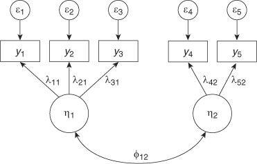
An example with five items (y1, …, y5), two factors (η1, η2), and five random measurement errors (ε1, …, ε5) is given in Figure 1; ϕ12 is the symbol for the covariance between the Factors 1 and 2.
The variance of the unique component can be further decomposed as  , where εs is the specific error variance due to the particular item (e.g., a specific item wording) and εe the random measurement error. In most cross-sectional studies, one cannot distinguish between these two kinds of errors because they are not separately identified. It is possible to separate these components only by using special designs like multitrait–multimethod or panel studies.
Figure 1 Visualization of a Factor Model With Five Observed and Two Latent Variables
Generally, one has to differentiate between EFA and CFA. EFA is used when there is no or not sufficient a priori knowledge about the number of factors and the relationship between items and constructs. CFA, in contrast, is used when researchers have concrete assumptions about the measurement model.
Exploratory Factor Analysis
EFA is a method used to detect the optimal number of factors that accounts for the correlation of items. Each factor is interpreted and named based on the items that have high loadings on this factor. Its character is inductive as the number of factors, the amount of correlations between factors, and the assignments between items and factors are performed empirically without a precise deductive theoretical model. There is no unique solution for the relation between observed items and latent factors. There are two different approaches to the factor model—(a) common-factor model and (b) principal component analysis—and each implies different substantive assumptions. In the common-factor model, it is assumed that every item is measured with some error. Therefore, the common-factor model is most appropriate in survey research, where items are always measured with some error. However, in the principal component model, the researcher assumes that there is no measurement error in the items. All analyses are based on correlation matrices as input.
EFA is performed in five steps:
- Factor extraction: The method that is most often used is the method of principal axis factoring and is based on the computation of the eigenvalues and vectors of the correlation matrix between all measured variables. Its goal is the maximization of the variance of each successively extracted factor.
- Number of factors: Different procedures determine the number of factors: (a) According to the Kaiser-Guttman criterion, the number of factors should correspond to the number of eigenvalues of the full input correlation matrix that exceed one. (b) The scree plot is a graph of each eigenvalue plotted in descending order. The number of factors is determined by visual inspection by observing whether, suddenly, the plot shows no real difference between the last two eigenvalues in the scree plot. (c) In parallel analysis, a second factor analysis is calculated with a random data set with the same numbers of variables and cases as in the original analysis. Only the factors with higher eigenvalues than the factors of the random data are accepted. (d) In maximum likelihood estimation, one studies the amount of residuals left over after introducing more factors and evaluates them by goodness-of-fit tests of the whole model.
- Communality estimation as a measure for the common variance of every item: The most often used method for an initial estimate is the squared multiple correlation of one item with all other items. Depending on the number of factors extracted, the final solution contains the explained variance of every item.
- Factor rotation: The goal of rotation is to achieve “a simple structure” that allows a good interpretation of the resulting solution. Rotations can be orthogonal, assuming that there are no correlations between factors (e.g., varimax, quartimax, and equimax), or oblique (e.g., promax, oblimin), assuming that there exist correlations between factors. In the case of correlated factors, the factor loadings of items on factors contained in the pattern factor matrix represent standardized partialized regression coefficients. In the case of noncorrelated factors, these coefficients are simply correlation coefficients between items and factors. The factor structure matrix contains the simple bivariate correlations between items and constructs. The values differ from the factor pattern matrix only if factors are correlated.
- Factor score estimation: As a final step, one may be interested in estimating the factor scores. The factor scores are often used as weights for raw scores in the computation of indices that are used in subsequent analyses.
Confirmatory Factor Analysis
In contrast to EFA, in CFA, a theoretical model is needed that contains a series of a priori hypotheses. These hypotheses should be drawn from the substantive literature. For example, in the theory of values of Shalom Schwartz, 10 values are postulated and theoretically derived. Therefore, the 10 theoretical constructs can be formalized and tested as latent variables in a CFA model. However, it is not definitely determined in the literature which and how many dimensions and items are adequate to measure the concepts of nationalism and patriotism and whether one can differentiate between them. The hypotheses in a CFA model refer to the following aspects of a measurement model: (a) determination of the number of factors, (b) assumption regarding whether the factors are correlated or not, (c) determination of which items load on which factor and where to set loadings a priori to zero, and (d) assumptions about the correlations of the errors. CFA allows the specification and testing of these assumptions. It is possible to fix parameters to a certain value or to constrain parameters that are set equal to other parameters. One assumes that the expected value of random measurement error is zero (εs = 0) and the correlation of the random measurement error with the latent variable (factor) is also zero. Furthermore, it is necessary to fix one of the loadings to one or to standardize the variance of the latent variable to reach identification of the model, that is, to achieve a unique solution.
...
- Comparative Politics, Theory, and Methods
- Anarchism
- Anarchy
- Breakdown of Political Systems
- Cabinets
- Censorship
- Central Banks
- Change, Institutional
- Charisma
- Citizenship
- Collaboration
- Comparative Methods
- Comparative Politics
- Competition, Political
- Conditionality
- Constitutional Engineering
- Corporativism
- Decentralization
- Democracy, Types of
- Discursive Institutionalism
- Elites
- Environmental Issues
- Executive
- Government
- Historical Sociology
- Human Rights, Comparative Perspectives
- Hybrid Regimes
- Institutionalization
- Institutionalization
- Institutions and Institutionalism
- Interest Groups
- Irredentism
- Labor Movement
- Leadership
- Legitimacy
- Military Rule
- Monarchy
- Neo-Patrimonialism
- Neo-Weberian State
- Oligarchy
- Path Dependence
- Personalization of Politics
- Pillarization
- Political Integration
- Political Science, International
- Political Systems, Types
- Politics of Language
- Presidentialism
- Prospect Theory
- Qualitative Comparative Analysis
- Referenda
- Reform
- Regime (Comparative Politics)
- Regionalism
- Regionalization
- Representation
- Republic
- Republicanism
- Responsibility
- Responsiveness
- Revolution
- Rule of Law
- Secession
- Semipresidentialism
- Separation of Powers
- Social Movements
- Socialist Systems
- Stability
- State
- State, Virtual
- Terrorist Groups
- Totalitarian Regimes
- Welfare Policies
- Welfare State
- Case and Area Studies
- Area Studies
- Authoritarian Regimes
- Case Studies
- Caudillismo
- Communist Systems
- Comparative Methods
- Comparative Politics
- Cross-National Surveys
- Democracy: Chinese Perspectives
- Democracy: Middle East Perspectives
- Democracy: Russian Perspectives
- Fascist Movements
- Multiculturalism
- Populist Movements
- Postcommunist Regimes
- Regional Integration (Supranational)
- Subnational Governments
- Democracy and Democratization
- Accountability
- Accountability, Electoral
- Accountability, Interinstitutional
- Change, Institutional
- Citizenship
- Civil Service
- Coalitions
- Collaboration
- Colonialism
- Competition, Political
- Conditionality
- Constitutional Engineering
- Constitutionalism
- Corruption, Administrative
- Credible Commitment
- Democracy, Direct
- Democracy, Quality
- Democracy, Types of
- Democracy: Chinese Perspectives
- Democracy: Middle East Perspectives
- Democracy: Russian Perspectives
- Democratization
- Developing World and International Relations
- Development Administration
- Development, Political
- Empowerment
- Federalism
- Foreign Aid and Development
- Governance
- Governance, Good
- Groupthink
- Human Development
- Liberalization
- Modernization Theory
- Monarchy
- Nation Building
- Opposition
- Peasants' Movements
- Pluralist Interest Intermediation
- Postcolonialism
- Postmaterialism
- Representation
- Responsibility
- Responsiveness
- Responsiveness of Bureaucracy
- Rule of Law
- Self-Determination
- Semipresidentialism
- State Collapse
- State Failure
- State Formation
- Sustainable Development
- Traditional Rule
- Transition
- Transitional Justice
- Decision Making in Democracies
- Cost–Benefit Analysis
- Delegation
- Deliberative Policy Making
- Election by Lot
- Election Observation
- Election Research
- Elections, Primary
- Elections, Volatility
- Electoral Behavior
- Electoral Campaigns
- Electoral Geography
- Electoral Systems
- Electoral Turnout
- Executive
- Judicial Independence
- Judicial Systems
- Lobbying
- Parliamentary Systems
- Parliaments
- Participation
- Participation, Contentious
- Referenda
- Separation of Powers
- Voting Rules, Electoral, Effects of
- Voting Rules, Legislative
- Epistemological Foundations
- Behavioralism
- Biology and Politics
- Causality
- Concept Formation
- Conditions, Necessary and Sufficient
- Constructivism
- Constructivism in International Relations
- Critical Theory
- Critical Theory in International Relations
- Culturalism
- Democracy, Theories of
- Epistemic Communities
- Epistemological and Methodological Foundations
- Ethics
- Feminist Theory in International Relations
- Functionalism
- Historical Sociology
- Idealism
- Ideology
- Institutional Theory
- Institutions and Institutionalism
- Logic of Appropriateness
- Methodology
- Multiculturalism
- Neoliberal Institutionalism
- Neoliberalism
- Paradigms in Political Science
- Positivism
- Quantitative Versus Qualitative Methods
- Rationalism, Critical
- Rationality, Bounded
- Systems Theory
- Utilitarianism
- Gender and Race/Ethnicity
- International Relations
- Balance of Power
- Colonialism
- Constructivism in International Relations
- Containment
- Critical Theory
- Critical Theory in International Relations
- Democratic Peace
- Dependency Theory
- Developing World and International Relations
- Domestic Politics and International Relations
- Empire
- Europe as an International Actor
- Foreign Aid and Development
- Foreign Policy Analysis
- Governance, Global
- Human Rights in International Relations
- Indigenous Peoples' Rights
- Intergovernmentalism
- International Law
- International Organizations
- International Regimes
- International Relations as a Field of Study
- International Relations, Theory
- International System
- International Trade
- Intervention
- Intervention, Humanitarian
- Judicialization of International Relations
- Mediation in International Relations
- Multilateralism
- Nongovernmental Organizations (NGOs)
- Normative Theory in International Relations
- Political Science, International Institutionalization
- Postmodernism in International Relations
- Psychological Explanations of International Politics
- Realism in International Relations
- Superpower
- Peace, War, and Conflict Resolution
- Alliances
- Arms Race
- Bilateralism
- Bipolarity and Multipolarity
- Civil War
- Collective Security
- Conflict Resolution
- Conflicts
- Détente
- Diplomacy
- Disarmament
- Domestic Politics and International Relations
- Empire
- Foreign Policy Analysis
- Genocide
- Imperialism
- Intervention
- Intervention, Humanitarian
- Judicial Decision Making
- Judicialization of International Relations
- Mediation in International Relations
- Militias
- Multilateralism
- National Interest
- Natural Resources
- Neutrality
- Pacifism
- Participation, Contentious
- Peace
- Peacekeeping
- Positive Peace
- Power and International Politics
- Preemptive War
- Psychological Explanations of International Politics
- Sanctions
- Secession
- Security and Defense Policy
- Security Cooperation
- Security Dilemma
- Sovereignty
- Strategic (Security) Studies
- Superpower
- Territory
- Terrorism, International
- Transatlantic Relations
- Unilateralism
- United Nations
- Violence
- War and Peace
- Warlords
- Westphalian Ideal State
- World Systems Theory
- Political Economy
- Capitalism
- Central Banks
- Class, Social
- Cost–Benefit Analysis
- Economic Policy
- Economic Statecraft
- Economic Theories of Politics
- Foreign Aid and Development
- Inequality, Economic
- International Monetary Fund (IMF)
- International Political Economy
- Labor Movement
- Market Economy
- Market Failure
- Monetary Relations
- Multilateralism
- Multinational Corporations (MNCs)
- Nongovernmental Organizations (NGOs)
- Policy, Employment
- Political Economy
- Privatization
- Property
- Protectionism
- Public Budgeting
- Public Employment
- Public Goods
- Redistribution
- Social Stratification
- Sustainable Development
- Tax Policy
- Trade Liberalization
- Traditional Rule
- Tragedy of the Commons
- Transaction Costs
- Transformation, Economic
- Welfare Policies
- Welfare State
- World Bank
- World Trade Organization (WTO)
- Political Parties
- Christian Democratic Parties
- Cleavages, Social and Political
- Communist Parties
- Conservative Parties
- Green Parties
- Liberal Parties
- One-Party Dominance
- Parties
- Party Finance
- Party Identification
- Party Linkage
- Party Manifesto
- Party Organization
- Party System Fragmentation
- Party Systems
- Social Democracy
- Socialist Parties
- Political Philosophy/Theory
- African Political Thought
- Anarchism
- Charisma
- Communism
- Communitarianism
- Conservatism
- Constitutionalism
- Contract Theory
- Democracy, Theories of
- Discursive Institutionalism
- Ethics
- Fascism
- Fundamentalism
- Greek Philosophy
- Idealism in International Relations
- Liberalism
- Liberalism in International Relations
- Libertarianism
- Liberty
- Maoism
- Marxism
- Mercantilism
- Nationalism
- Neoliberal Institutionalism
- Neoliberalism
- Normative Political Theory
- Normative Theory in International Relations
- Pacifism
- Pluralism
- Political Class
- Political Philosophy
- Political Psychology
- Political Theory
- Postmodernism in International Relations
- Realism in International Relations
- Revisionism
- Rights
- Secularism
- Socialism
- Stalinism
- Statism
- Theocracy
- Utilitarianism
- Utopianism
- Equality and Inequality
- Formal and Positive Theory
- Theorists
- Political Sociology
- Alienation
- Anomia
- Apathy
- Attitude Consistency
- Beliefs
- Civic Culture
- Civic Participation
- Corporativism
- Credible Commitment
- Diaspora
- Dissatisfaction, Political
- Elections, Primary
- Electoral Behavior
- Elitism
- Empowerment
- Hegemony
- Historical Memory
- Intellectuals
- International Public Opinion
- International Society
- Media, Electronic
- Media, Print
- Migration
- Mobilization, Political
- Neo-Corporatism
- Networks
- Nonstate Actors
- Participation
- Participation, Contentious
- Party Identification
- Patriotism
- Pillarization
- Political Communication
- Political Culture
- Political Socialization
- Political Sociology as a Field of Study
- Popular Culture
- Power
- Schema
- Script
- Social Capital
- Social Cohesion
- Social Dominance Orientation
- Solidarity
- Subject Culture
- Support, Political
- Tolerance
- Trust, Social
- Values
- Violence
- Public Policy
- Advocacy
- Advocacy Coalition Framework
- Agencies
- Agenda Setting
- Bargaining
- Common Goods
- Complexity
- Compliance
- Contingency Theory
- Cooperation
- Coordination
- Crisis Management
- Deregulation
- Discretion
- Discursive Policy Analysis
- Environmental Policy
- Environmental Security Studies
- Europeanization of Policy
- Evidence-Based Policy
- Immigration Policy
- Impacts, Policy
- Implementation
- Joint-Decision Trap
- Judicial Decision Making
- Judicial Review
- Legalization of Policy
- Metagovernance
- Monitoring
- Neo-Weberian State
- New Public Management
- Organization Theory
- Policy Advice
- Policy Analysis
- Policy Community
- Policy Cycle
- Policy Evaluation
- Policy Formulation
- Policy Framing
- Policy Instruments
- Policy Learning
- Policy Network
- Policy Process, Models of
- Policy, Constructivist Models
- Policy, Discourse Models
- Policy, Employment
- Prospect Theory
- Reorganization
- Risk and Public Policy
- Self-Regulation
- Soft Law
- Stages Model of Policy Making
- Think Tanks
- Tragedy of the Commons
- Transaction Costs
- Public Administration
- Administration
- Administration Theory
- Audit Society
- Auditing
- Autonomy, Administrative
- Budgeting, Rational Models
- Bureaucracy
- Bureaucracy, Rational Choice Models
- Bureaucracy, Street-Level
- Civil Service
- Corruption, Administrative
- Effectiveness, Bureaucratic
- Governance
- Governance Networks
- Governance, Administration Policies
- Governance, Informal
- Governance, Multilevel
- Governance, Urban
- Groupthink
- Health Policy
- Intelligence
- Pay for Performance
- Performance
- Performance Management
- Planning
- Police
- Politicization of Bureaucracy
- Politicization of Civil Service
- Public Budgeting
- Public Employment
- Public Goods
- Public Office, Rewards
- Regulation
- Representative Bureaucracy
- Responsiveness of Bureaucracy
- Secret Services
- Security Apparatus
- Qualitative Methods
- Analytic Narratives: Applications
- Analytic Narratives: The Method
- Configurational Comparative Methods
- Data, Textual
- Discourse Analysis
- Ethnographic Methods
- Evaluation Research
- Fuzzy-Set Analysis
- Grounded Theory
- Hermeneutics
- Interviewing
- Interviews, Elite
- Interviews, Expert
- Mixed Methods
- Network Analysis
- Participant Observation
- Process Tracing
- Qualitative Comparative Analysis
- Quantitative Versus Qualitative Methods
- Thick Description
- Triangulation
- Quantitative Methods
- Aggregate Data Analysis
- Analysis of Variance
- Boolean Algebra
- Categorical Response Data
- Censored and Truncated Data
- Cohort Analysis
- Correlation
- Correspondence Analysis
- Cross-National Surveys
- Cross-Tabular Analysis
- Data Analysis, Exploratory
- Data Visualization
- Data, Archival
- Data, Missing
- Data, Spatial
- Event Counts
- Event History Analysis
- Experiments, Field
- Experiments, Laboratory
- Experiments, Natural
- Factor Analysis
- Fair Division
- Fuzzy-Set Analysis
- Granger Causality
- Graphics, Statistical
- Hypothesis Testing
- Inference, Ecological
- Interaction Effects
- Item–Response (Rasch) Models
- Logit and Probit Analyses
- Matching
- Maximum Likelihood
- Measurement
- Measurement, Levels
- Measurement, Scales
- Meta-Analysis
- Misspecification
- Mixed Methods
- Model Specification
- Models, Computational/Agent-Based
- Monte Carlo Methods
- Multilevel Analysis
- Nonlinear Models
- Nonparametric Methods
- Panel Data Analysis
- Political Risk Analysis
- Prediction and Forecasting
- Quantitative Methods, Basic Assumptions
- Quantitative Versus Qualitative Methods
- Regression
- Robust Statistics
- Sampling, Random and Nonrandom
- Scaling
- Scaling Methods: A Taxonomy
- Selection Bias
- Simultaneous Equation Modeling
- Statistical Inference, Classical and Bayesian
- Statistical Significance
- Statistics: Overview
- Structural Equation Modeling
- Survey Research
- Survey Research Modes
- Time-Series Analysis
- Time-Series Cross-Section Data and Methods
- Triangulation
- Variables
- Variables, Instrumental
- Weighted Least Squares
- Religion
- Loading...
Get a 30 day FREE TRIAL
-
 Watch videos from a variety of sources bringing classroom topics to life
 -
Read modern, diverse business cases
-
Explore hundreds of books and reference titles

Read next

More like this
Sage Recommends
We found other relevant content for you on other Sage platforms.
Have you created a personal profile? Login or create a profile so that you can save clips, playlists and searches