Analysis of Variance

Analysis of variance (ANOVA) is a method for decomposing variance in a measured outcome into variance that can be explained, such as by a regression model or an experimental treatment assignment, and variance that cannot be explained, which is often attributable to random error. Using this decomposition into component sums of squares, certain test statistics can be calculated that can be used to describe the data or even justify model selection. Lab experiments have become increasingly popular in political science, and ANOVA is a useful tool for analyzing such experiments. In recent years, there have been a number of laboratory experiments on the effects of campaigning and media advertising. Nicolas Valentino, Vincent Hutchings, and Ismail White (2002), Diana Mutz and Byron Reeves (2005), and Ted Brader (2005) have all performed lab experiments that aim to determine the effect that campaigning and advertising in media have on voters views and decisions. All three experiments employ an ANOVA to control for observable characteristics, interactions between treatment regimes, and significance of the relative effectiveness of treatments. This [Page 63]entry discusses ANOVA and its applications in greater detail.

In the familiar regression context, the “sum of squares” (SS) can be decomposed as follows. Assuming that Yi is individual i's outcome, is the mean of the outcomes, Ŷi is individual i's fitted value based on the ordinary least squares (OLS) estimates, and ei is the resulting residual,

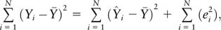
where

is the total sum of squares,

refers to the variance explained by the regression, and

is the variance due to the error term, also known as the unexplained variance. Commonly, we would write this decomposition as

The equations above show how the total variance in the observations can be decomposed into variance that can be explained by the regression equation and variance that can be attributed to the random error term in the regression model.

ANOVA is not restricted to use with regression models. The concept of decomposing variance can be applied to other models of data, such as an experimental model. The following is the decomposition of a one-way layout experimental design in which an experimenter randomly assigns observations to one of I treatment assignments. Each treatment assignment has J observations assigned to it. In the case of a randomized controlled trial with only one treatment regime and N subjects randomly assigned to treatment with half a probability, this would mean that I = 2, one treated group and one control group, where each group has size J. In this framework, the variance decomposition would be as follows:

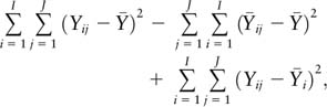
where

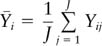
is defined as the average response under the Ith treatment and

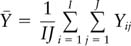
is defined as the overall average of all observations, regardless of treatment assignment. Commonly, this sum of squares expression is written as

where SSbetween refers to the part of the variance that can be attributed to the different treatment assignments and SSwithin refers to the variance that can be described by the random error within a treatment assignment. From this, we can see that SSbetween and SSregression, from the regression framework, both refer to the explained variance. SSwithin and SSerror both refer to the unexplained variance.

...