Housing Demand

Early Demand Analyses

Economists have long sought to identify determinants of housing demand. Unlike most economic goods, dwellings do not have easily identified units of service or easily identified prices for those services. As a result, analysts often concentrated on aggregate housing expenditures as fractions of income and on the impacts of changes in incomes and prices on these expenditures.

Richard Muth and Margaret Reid found that 1% increases in income were accompanied by substantial increases in housing expenditures. Economists standardize these measures as elasticities, with income elasticity as the following:

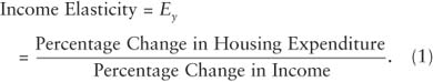
[Page 356]The matching 1% increases of income and expenditures imply constant income shares, or income elasticities, of about +1.0 (or in Reid's analyses, even higher).

Similarly, looking across groups of households, or countries with similar incomes, housing expenditure shares seemed to be about constant regardless of the prices. Similar to the income elasticity, the price elasticity is as follows:

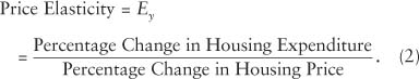
In demand theory, constant shares imply a price elasticity of −1.0, where higher prices lead to an equal offset in quantity purchased.

Combining these estimates with emerging urban economic theory explained the incongruity of poor people living in central cities on high-priced land in high-priced housing, whereas more affluent people commuted farther as they demanded more and cheaper land (housing) in the suburbs. However, the aggregate analyses did not predict how individual families would react to changes in economic variables, such as price or income, or to changed demographic conditions, such as larger (or smaller) household size. The aggregate analyses did not address why some families rented and others owned, and they did not provide good guidance into how to implement demand-related housing policies.

Microlevel Analyses

With improved data and computing methods, housing analysts focused on microeconomic and econometric analyses. Modern housing demand analysis starts with the identity that housing is either owned or rented and examines the behavioral determinants:

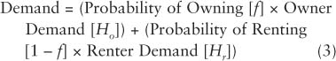
Analysts recognize that owner demand, renter demand, and probability of owning have behavioral components related to income (Y), owner or renter price (Po or P r), and demographics (D). An increase in income affects the quantities purchased by owners (H o), quantities purchased by renters (H r), and the decision of whether to own or rent (f). This income effect can be parsed into three parts:

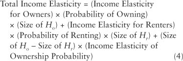
The first two effects look at owner and renter demand separately, and the third recognizes that owner housing was traditionally “bigger” than renter housing and gave a bigger “bump” to housing demand. Similar decompositions apply to prices and demographic effects.

Measuring microlevel housing demand required advances in applied techniques. Neither income nor price is unambiguous. Because of the high transactions costs of moving, most analysts relate demand to permanent income, following Milton Friedman. Observed income Y is the sum of permanent Y P and transitory Y T income components, and econometric theory shows how permanent income can be estimated as the return to human and nonhuman capital. Appropriate decomposition often doubles estimated “observed income” elasticities.

...