Spatial Heterogeneity

A quantitative model in which the relationships between variables depend on location is said to be spatially heterogeneous. Quantitative geographical models assume certain mathematical relationships exist between the locations and attributes of geographical entities. These relationships typically involve both a deterministic and a random component. A basic example of this is a standard linear regression model

where y is an attribute that depends on {x1… xj } through the linear coefficients {a0… aj } and the [Page 415]random term ∊i. Typically, it is assumed that the ∊i 's have a normal distribution and that they are independent. Of note in a model of this kind is the fact that the relationships are only between the attributes of the objects—location plays no role. Since the relationship between attributes is not dependent on location, this model is said to be spatially homogeneous. From the initial definition, a model not having this property is spatially heterogeneous. A large number of geographic models exhibit spatial heterogeneity.

One example is the geographically weighted regression (GWR) model. Here, the coefficients in Equation 1 are replaced by functions of the geographical coordinates of location in the study area (u, v), so that the model now becomes

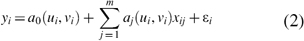
where (ui, vi) are the (u, v) coordinates for location i. Thus, the relationship between attributes now depends on geographical location. GWR models are usually calibrated by placing a kernel function around any given (u, v) and using this as a weighting scheme to calibrate a standard weighted least squares regression model, noting that if we choose a new (u, v) at which to calibrate the model, weights must change accordingly and the calibration rerun. Typically, coefficients are calibrated at the points (ui, vi) corresponding to the locations of the geographical objects or at points located on a regular grid covering the study area.

Another, perhaps subtler, form of spatial heterogeneity can be seen in extensions of the linear regression model

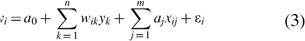
where the error terms ∊i are not considered as independent. In a number of spatial models, the y-variables are modeled as being correlated, with the degree of correlation depending on the proximity of the locations. One such model is the spatial autoregressive model where the wik is an indicator of proximity between objects i and k. For example, if the objects are geographical areas, wik is 1 if the areas are adjacent and 0 if they are not. To ensure the model is valid, wii is zero for all i. If W is the matrix formed by all wik 's, then for any given observation i, Equation 3 uses the ith row of W. Thus, since the equation for each i uses a different row of W, the model is spatially heterogeneous.

This example differs from the others, however, in that the above equation varies according to the relative proximities of all of the observations, whereas the first two examples depend on the absolute location of each location. The model underlying the statistical technique of kriging also has this property. In one sense, this kind of model does exhibit homogeneity—the relative proximity of two objects is always treated the same, regardless of their absolute location. In kriging, for example, the correlation between measurements taken at two vector locations x1 and x2 depends only on x1 − x2.

...