Spatial Autocorrelation

Spatial autocorrelation is a spatial measure that evaluates how dispersed or clustered points are distributed in space and whether or not this distribution has occurred by chance. Unlike other spatial methods for detecting spatial patterns of point distribution without considering their attributes, such as Quadrat analysis and the Nearest Neighbor method, spatial autocorrelation also characterizes how similar these points are with respect to their attribute values. There are two typical spatial autocorrelation statistics: Moran's I and Geary's C. Both Moran's I and Geary's C measure the proximity of locations and evaluate the similarity of attributes.

If the statistics show more positive correlation than would be expected from a randomly distributed pattern, points with similar attribute values are closely distributed in space (Figure 1A), whereas negative spatial autocorrelation statistics indicate that closely associated points are more dissimilar. A chess board is an example of negative spatial autocorrelation (Figure 1B); every black cell is adjacent to white squares, indicating that the neighbors are not similar. Care should be taken when using spatial autocorrelation, as it is related to the scale of the data.

Moran's I can be computed as

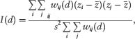
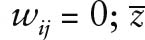
where wij is the weight at distance d such that wij = 1 if point j is within distance d from point i, otherwise wij = 0;

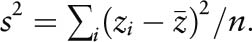
is the mean attribute value; s2 is the variance of the attribute values and can be calculated as

Moran's I varies from +1.0 for perfect positive correlation to—1.0 for perfect negative correlation.

Geary's C is calculated from the following:

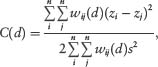
where wij is the weight; s2 is the variance of z values and can be computed as.

The weight, wij, only considers the values 0 and 1, [Page 2608]as mentioned above. A typical Geary C value ranges between 0 and 2. A value of less than 1.0 implies positive autocorrelation, 1.0 implies no autocorrelation, and values of greater than 1.0 imply negative autocorrelation.

Figure 1 Hypothetical images with (A) positive spatial autocorrelation and (B) negative spatial autocorrelation

Source: Authors.

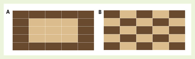
Figure 2 Hypothetical images with (A) hot spots and (B) cold spots

Source: Authors.

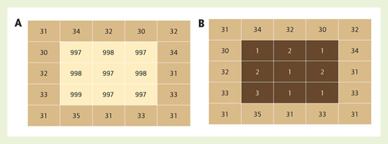
Similarly, another spatial autocorrelation approach called the Getis statistic (Gi) was developed to characterize the presence of hot spots (Figure 2A) and cold spots (Figure 2B), which are sets of clustered points with large or small attribute values, respectively.

The Getis statistic is computed as

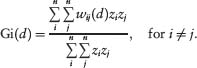
The Gi is also defined by a distance, d, within which areal units can be regarded as neighbors of i. The weight wij(d) is 1 if areal unit j is within d and is 0 otherwise. Some of the zi, zj pairs will not be considered in the calculation of the numerator if i and j are more than d away from each other.