
Summary
Contents
Subject index
Geographic information systems (GIS) have become increasingly important in helping us understand complex social, economic, and natural dynamics where spatial components play a key role. The critical algorithms used in GIS, however, are notoriously difficult to both teach and understand, in part due to the lack of a coherent representation. GIS Algorithms attempts to address this problem by combining rigorous formal language with example case studies and student exercises. Using Python code throughout, Xiao breaks the subject down into three fundamental areas: • Geometric Algorithms • Spatial Indexing • Spatial Analysis and Modelling With its comprehensive coverage of the many algorithms involved, GIS Algorithms is a key new textbook in this complex and critical area of geography.
GDAL/OGR and PySAL
Many Python packages have been developed to handle geospatial data. In this appendix we introduce two sets of libraries for different purposes. GDAL (Geospatial Data Abstraction Library) is a powerful library that can be used to support various tasks in handling geospatial data sets. GDAL is designed to handle raster data and supports about 100 raster formats.1 GDAL represents a major advance in free and open source GIS. As a component of GDAL, OGR supports vector data formats. OGR used to mean OpenGIS Simple Features Reference Implementation, but the OGR library does not fully comply with the OpenGIS Simple Features Specification of the Open GIS Consortium (OGC) and therefore was not approved by the OGC. As a consequence, OGR today technically does not stand for anything. In general, OGR supports many vector formats2 such as shapefiles, personal geodatabases, ArcSDE, MapInfo, GRASS, TIGER/Line, SDTS, GML, and KML. It also supports many database connections, including MySQL, PostgreSQL, and Oracle Spatial. More information about GDAL and OGR can be found on their website.3 GDAL/OGR was not initially developed as a Python library, but many programming languages support GDAL/OGR, including Python. In that sense, we are using a Python wrapper of the binary library of GDAL/OGR, which to some extent will have consequences on the performance of the code.
The second library is an open source software package called PySAL (Python Spatial Analysis Library) that has been used in a wide range of applications of spatial data.4 Different from GDAL/OGR, PySAL is developed in Python and supports a wide range of spatial analysis applications. PySAL has its own core data structure that supports file input and output. A key component of PySAL is spatial weights that are central in many spatial analysis methods.
In this appendix, we will go through some basic features to demonstrate how these powerful geospatial libraries can help us implement and understand many of the algorithms covered in this book. This appendix is mainly based on coding, with a lot of comments. Some of the lines included here are for instructional purposes and therefore may not be necessary in all cases. However, they should provide a good context in which to understand the functionality of GDAL/ORG and PySAL. We do not intend to explain the meaning of each and every line since it should be relatively straightforward to understand (especially with the extensive comments for most parts of the code). For more applications and details of the use of GDAL/OGR library, there is an online Python GDAL/ORG Cookbook.5 PySAL has its own tutorials6 that include details of how to use the library.
There is a great deal we can do with the power of GDAL/OGR and PySAL because these libraries give us a convenient way to convert geospatial data in any format into any data structures. Almost every algorithm introduced in this book can be plugged in here. We should take this opportunity to test and explore those algorithms using our own data.
Both GDAL/OGR and PySAL can be installed on different operating systems. We do not discuss the installation process here since the websites of these libraries provide detailed information.
B.1 OGR
To use OGR, we typically should start with the following lines, where we show how OGR works for a shapefile. In the following example, we assume there is a polygon shapefile called uscnty48area.shp existing in a folder called data in the upper level of the current working directory. To make it work for new data, we will need to have a polygon shapefile and make sure we know the path to that file. We focus on polygon shapefiles here. For other types of shapefiles (e.g., polyline), the processes are similar though the details will be different. We have an example of the use of a polyline shapefile (world coastlines) in Chapter 2. The last line in the following code should return False, indicating successful reading of the shapefile.

B.1.1 Attributes
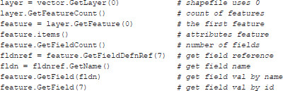
The variable vector instantiated in the previous code lets us access the information stored in the shapefile. A general procedure is to go down the hierarchy of file > layer > feature to access different types of information. For a shapefile, one file only contains one layer, which in turn contains multiple features. Below are the lines of code for accessing the attributes associated with a feature.
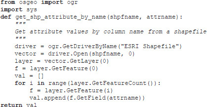
We can write a short function (getattr.py) that returns a list of values in an attribute in a shapefile. We will use this function later in Section B.3.
B.1.2 Geometry and coordinates
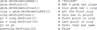
We will now see how to retrieve the geometry and coordinates from the shapefile we just loaded. We only show how to get points of one polygon, but it is of course possible to get points for all polygons using a loop, as we will show later.

B.1.3 Projecting points
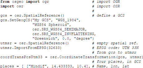
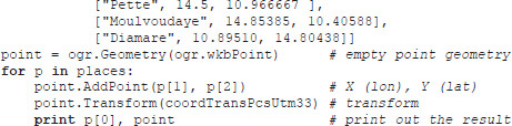
We can transform a set of points in a geographic coordinate system (GCS) expressed in longitudes and latitudes into a projected coordinate system. Suppose we have a few locations from northern Cameroon that are recorded in WGS84 datum format, and we want to transform them into UTM zone 33N format. Here we will use the OSR (OGRSpatialReference) library, an OGR module for processing spatial reference systems, to transform between coordinate systems. OSR is based on the PROJ.4 Cartographic Projections Library.7 The general flow of work is to start by defining the source coordinate system, which is what we call gcs in the following code. Then we define the target coordinate system, called utmsr below. There are different ways to define a projected coordinate system, and we choose the easiest way using the EPSG code that is uniquely assigned to UTM 33N. With these two coordinate systems, we can define a transformation using the OSR function CoordinateTransformation, and here we name the transformation coordTransPcsUtm33. The known coordinates we have for the four locations in Cameroon are stored in a list of lists where the string in each element list refers to a place name. We first need to convert these coordinates into a point geometry in OGR and then we can simply use the Transform function to do the coordinate system transformation.
B.1.4 Projecting and writing geospatial data
Now we turn to our shapefile that is in a GCS and this time we will project it to the Albers equal-area conic projection that is commonly used for the conterminous United States. Our shapefile comes with a .prj file and we can read the spatial reference information directly from there. The general idea here is to find each point and transform it to a new coordinate system and then write it to a ring, which is in turn added into a polygon feature. We save the transformed data into a new shapefile.
A general polygon in a shapefile may have holes, where each hole and the outline polygon are called rings. However, many counties in our data also have islands in a river or lake and these islands are not holes. In this case, they are organized as multipolygons. As the name suggests, each multipolygon includes a set of polygons, and each of those polygons may still contain holes. To streamline the process of handling such data, we design a specific function trans_rings that retrieves every ring in the input geometry that must be a polygon, which must not be a multipolygon but can have holes. (Having holes or not does not affect how this function works because holes and the outline polygon are all treated as rings and a polygon will have at least one ring.) This function returns a new polygon that contains transformed points. This polygon is then added into the feature for the new shapefile. For a feature that is only a simple polygon (with or without holes), we call this function once and get a new polygon. For a multipolygon feature, we will need to call this function multiple times, each time for a polygon in the multipolygon. Every time a new polygon is added, we create a new feature and add the polygon into the feature.
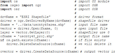
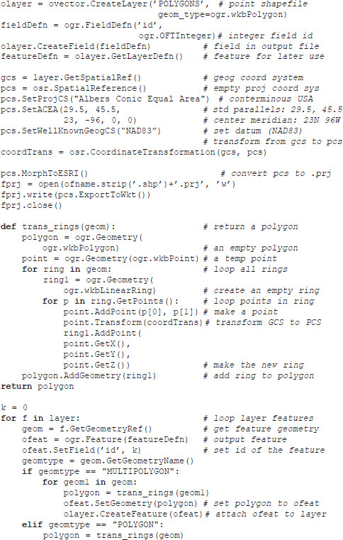
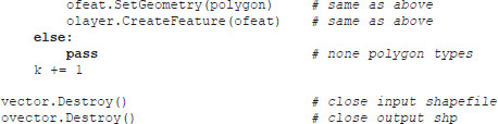
Figure B.1 Projecting spatial data. Left: original data in GCS. Right: data projected into Albers equal-area conic projection
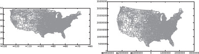
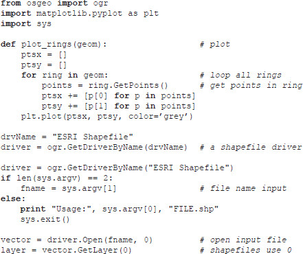
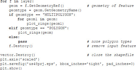
The result is shown in Figure B.1. The two maps in this figure are drawn using Matplotlib using the following Python code (draw_shp_polygons.py).
B.1.5 Adjacency matrix
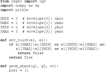
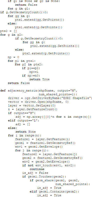
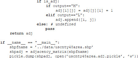
Our final project using OGR is to create an adjacent matrix for a polygon shapefile. The procedure is simple: we continuously check each pair of polygons and test if they touch each other or one contains another. We use the OGR Touches and Contains functions to do so. To speed up the process, we design a function called env_touch to test if the bounding boxes (envelopes) of two polygons touch each other. We can write a function called geom_touch to test whether two OGR geometry objects touch each other by sharing a specified number of points (in parameter n0).
The adjacency_matrix function takes three input parameters: the path to the shapefile, the output format (M for matrix and L for list), and the number of shared points for polygons to be considered as adjacent (default is 1). In the test of the function, we use the US county shapefile and dump the final result in matrix form in a Python pickle file. In Python, pickle is a standard way of translating complicated objects so that we can store them in a text file and restore them for future use. The pickle file stored here is used in our main text (Section 9.2) for calculating Moran’s I.
B.2 GDAL
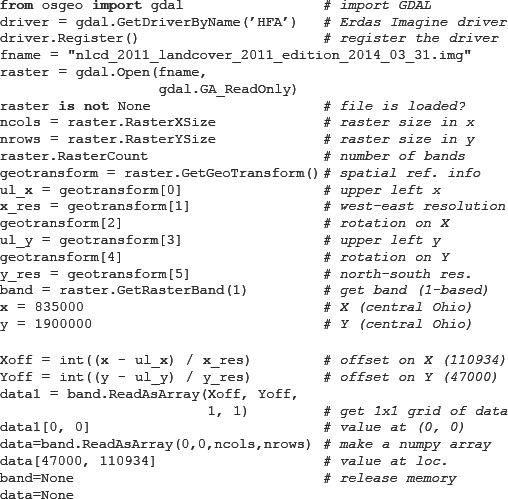
We now turn to GDAL to explore a few ways to access raster data. In this example we use the 2011 National Land Cover Database (NLCD) to demonstrate the use of GDAL. Similarly to OGR, we will need a driver to start using raster data, but in GDAL we also need to call the Register function before we can actually use it to open the raster file. Driver names (code) are available at http://www.gdal.org/formats_list.html. The NLCD we use here is stored in Erdas Imagine format (.img), and the GDAL code for that is HFA. The purpose here is to load the NLCD data into a NumPy array using the ReadAsArray function. Once the data are in an array format, which is an intuitive format for raster data, we can process them using many other methods such as the contagion metric (Section 9.4).
B.3 PySAL
PySAL covers a very wide range of topics in spatial analysis and beyond (Rey and Anselin, 2010). Here we demonstrate how to use it to calculate Moran’s I for an area data set. PySAL provides a lot of options to select the type of spatial weights. Here we use binary weights, meaning the weight between two polygons will be either 1 (adjacent) or 0 (non-adjacent). There are also a few different ways to compute the adjacency between polygons, and here we use the queen criterion, in which two polygons are adjacent if they share one or more points (the rook criterion, on the other hand, would require that they share an edge). Based on these choices, we will be able to compare the PySAL results with the code discussed in this book.
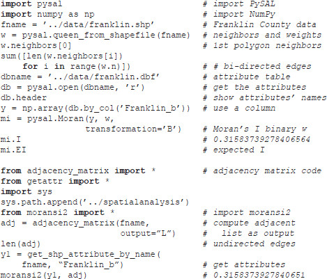
In Section 9.2, we introduced the calculation of Moran’s I based on an adjacency matrix (or list), which is equivalent to the binary weights determined using the queen criterion. The above code also tests the result of using the Moran’s I code in this book and the results are almost identical (readers who are interested in this example can examine the source code and explain what causes the very small difference between the two programs). To further validate the results, we can test the same data using the spdep package in R. To the precision reported in the R package, the result is 0.3158373928, which is consistent with the results obtained by the Python programs.
1 A full list of the supported formats can be found at http://www.gdal.org/formats_list.html
2 A full list of vector data formats supported under OGR can be found at http://www.gdal.org/ogr/ogr_formats.html
5http://pcjericks.github.io/py-gdalogr-cookbook/
- Loading...
Get a 30 day FREE TRIAL
-
 Watch videos from a variety of sources bringing classroom topics to life
 -
Read modern, diverse business cases
-
Explore hundreds of books and reference titles
Read next

More like this
Sage Recommends
We found other relevant content for you on other Sage platforms.
Have you created a personal profile? Login or create a profile so that you can save clips, playlists and searches